3d analysis and rendering of damage in a steel tension sample

This recipe demonstrate how to analyze the cavities in a steel sample deformed under tension loading.

Get the complete Python source code: steel_damage_analysis.py

The 3d data set is a 8 bits binary file with size 341x341x246. First you need to define the path to the 3d volume:

data_dir = '../../examples/data'
scan_name = 'steel_431x431x246_uint8'
scan_path = os.path.join(data_dir, scan_name + '.raw')

Then load the volume in memory thanks to the :pymicro:file:file_utils:HST_read function:

data = HST_read(scan_path, header_size=0)

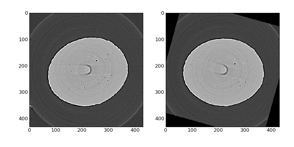
The reconstructed tomographic volume is not align with the cartesian axes, so rotate the volume by 15 degrees:

data = ndimage.rotate(data, 15.5, axes=(1, 0), reshape=False)

The result of these operations can be quickly observed using regular pyplot functions such as imshow. Here we look at slice number 87 where a ring artifact is present. We will take care of those later.

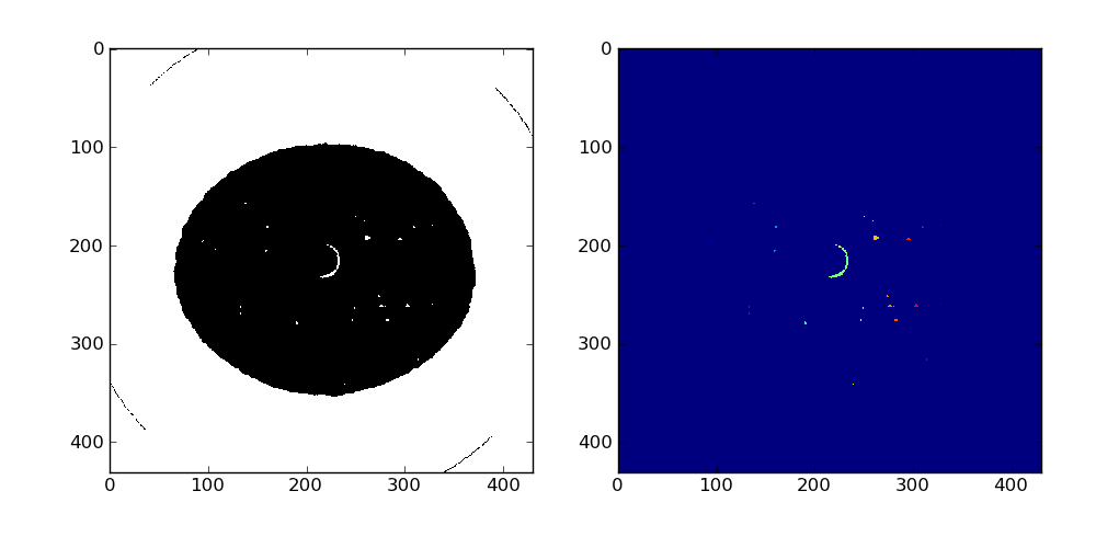
The entire volume is binarized using a simple threshold with the value 100:

data_bin = np.where(np.greater(data, 100), 0, 255).astype(np.uint8)

And cavities are labeled using standard scipy tools:

label_im, nb_labels = ndimage.label(data_bin)

3465 labels have been found, the result can be observed on slice 87 using pyplot:

We use a simple algorithm to remove ring articfacts (assuming the cavities are convex): the center of mass of each label is compute and if it does not lie inside the label, the corresponding voxels are set to 0. Here 11 rings were removed.

# simple ring removal artifact
coms = ndimage.measurements.center_of_mass(data_bin / 255, labels=label_im, \
                                           index=range(1, nb_labels + 1))
rings = 0
for i in range(nb_labels):
    com_x = round(coms[i][0])
    com_y = round(coms[i][1])
    com_z = round(coms[i][2])
    if not label_im[com_x, com_y, com_z] == i + 1:
        print 'likely found a ring artifact at (%d, %d, %d) for label = %d, value is %d' \
              % (com_x, com_y, com_z, (i + 1), label_im[com_x, com_y, com_z])
        data_bin[label_im == (i + 1)] = 0
        rings += 1
print 'removed %d rings artifacts' % rings

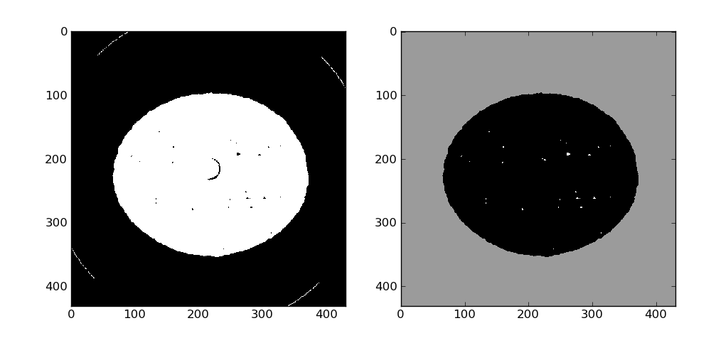
The outside of the sample needs a little love, it is by far the largest label here so after inverting the labeled image and running a binary closing it can be set to a fixed value (155 here) in the data_bin array.

print('labeling and using a fixed color around the specimen')
# the outside is by far the largest label here
mask_outside = (sizes >= ndimage.maximum(sizes))
print('inverting the image so that outside is now 1')
data_inv = 1 - label_im
outside = mask_outside[data_inv]
outside = ndimage.binary_closing(outside, iterations=3)
# fix the image border
outside[0:3, :, :] = 1;
outside[-3:, :, :] = 1;
outside[:, 0:3, :] = 1;

At this point the segmented volume can be written to the disk for later use using the HST_write function:

plt.subplots_adjust(left=0.1, right=0.95, top=0.95, bottom=0.1)