4 - Creating, getting and visualizing Image Groups and Image Fields

This Notebook will introduce you to:

1. what is an Image Group

2. the Image Group data model

3. how to create an image Group

4. the Image Field data model

5. how to add a field to an Image Group

6. how to get image groups and image fields

Note

Throughout this notebook, it will be assumed that the reader is familiar with the overview of the SampleData file format and data model presented in the first notebook of this User Guide of this User Guide.

I - SampleData Image Groups

SampleData Grids

In the last tutorial, the basic data item types that can be loaded into a SampleData dataset have been presented. They consist in various types of data arrays (numeric arrays, structured arrays, string arrays) and attributes, that can be stored in Groups to organize them.

However, the main focus of the class has been put on spatially organized data. This type of data, which includes field measurements, imaging techniques and numerical simulation outputs, is central to modern materials and microstructure science. Each of those outputs can be seen as a set of fields supported by a grid.

A grid is a set of nodes and elements that define a discretization of a geometrical domain. A field is a function defined on this geometrical domain. On the discrete grid, field are defined by an array containing the values that it takes at on grid nodes or grid elements. Hence, geometrical data and field data are intrinsically linked. Therefore, in addition to storing the data arrays containing the node/elements/fields values data, some geometrical organization connecting these data items must be stored as well in the datasets.

To connect data together within SampleData datasets, we can use Groups and Attributes (metadata). So, to handle spatially organized data, SampleData defines Grid groups, that have a specific data model (sub-groups, arrays and metadata). In addition to this, these group are syncrhronized with a Grid node in the XDMF dataset file, to ensure that the data stored in the Grid group can be visualized with its correct spatial organization in the Paraview software.

There are two types of Grid groups: Image groups, and Mesh groups. In this tutorial, we will learn everything that is to know on Image groups.

SampleData Images

As indicated by their name, Image Groups are a specific type of Grid group whose data model is adapted to store images. Images are 2D or 3D regular grids of pixels(2D)/voxels(3D), all having the same dimensions. To this pixel/voxel grid is also associated a node grid, composed by the vertexes of the pixels/voxels. Three types of Image Groups can be handled by SampleData:

1. emptyImage: an empty group that can be used to set the organization and metadata of the dataset before adding actual data to it (similar to empty data arrays, see tutorial 2, section IV)

2. 2DImage: a regular grid of pixels

3. 3DImage: a regular grid of voxels

An Image field is a data array that has one value associated to each pixel/voxel or each node of the image.

Hence, Image Groups contain metadata indicating the image topology, data arrays containing the image fields values, and metadata to synchronize with the XDMF Grid node associated to the Image. To explore in details this data model, we will once again open the reference test dataset of the SampleData unit tests, in the next section.

II - Image Groups Data Model

from pymicro.core.samples import SampleData as SD

from config import PYMICRO_EXAMPLES_DATA_DIR # import file directory path
import os
dataset_file = os.path.join(PYMICRO_EXAMPLES_DATA_DIR, 'test_sampledata_ref') # test dataset file path
data = SD(filename=dataset_file)

Let us print the content of the dataset to remember its composition:

print(data)

Dataset Content Index :
------------------------:
index printed with max depth `3` and under local root `/`

         Name : array                                     H5_Path : /test_group/test_array
         Name : group                                     H5_Path : /test_group
         Name : image                                     H5_Path : /test_image
         Name : image_Field_index                         H5_Path : /test_image/Field_index
         Name : image_test_image_field                    H5_Path : /test_image/test_image_field
         Name : mesh                                      H5_Path : /test_mesh
         Name : mesh_ElTagsList                           H5_Path : /test_mesh/Geometry/Elem_tags_list
         Name : mesh_ElTagsTypeList                       H5_Path : /test_mesh/Geometry/Elem_tag_type_list
         Name : mesh_ElemTags                             H5_Path : /test_mesh/Geometry/ElementsTags
         Name : mesh_Elements                             H5_Path : /test_mesh/Geometry/Elements
         Name : mesh_Field_index                          H5_Path : /test_mesh/Field_index
         Name : mesh_Geometry                             H5_Path : /test_mesh/Geometry
         Name : mesh_NodeTags                             H5_Path : /test_mesh/Geometry/NodeTags
         Name : mesh_NodeTagsList                         H5_Path : /test_mesh/Geometry/Node_tags_list
         Name : mesh_Nodes                                H5_Path : /test_mesh/Geometry/Nodes
         Name : mesh_Nodes_ID                             H5_Path : /test_mesh/Geometry/Nodes_ID
         Name : mesh_Test_field1                          H5_Path : /test_mesh/Test_field1
         Name : mesh_Test_field2                          H5_Path : /test_mesh/Test_field2
         Name : mesh_Test_field3                          H5_Path : /test_mesh/Test_field3
         Name : mesh_Test_field4                          H5_Path : /test_mesh/Test_field4

Printing dataset content with max depth 3
  |--GROUP test_group: /test_group (Group)
     --NODE test_array: /test_group/test_array (data_array) (   64.000 Kb)

  |--GROUP test_image: /test_image (3DImage)
     --NODE Field_index: /test_image/Field_index (string array) (   63.999 Kb)
     --NODE test_image_field: /test_image/test_image_field (field_array) (   63.867 Kb)

  |--GROUP test_mesh: /test_mesh (3DMesh)
     --NODE Field_index: /test_mesh/Field_index (string array) (   63.999 Kb)
    |--GROUP Geometry: /test_mesh/Geometry (Group)
       --NODE Elem_tag_type_list: /test_mesh/Geometry/Elem_tag_type_list (string array) (   63.999 Kb)
       --NODE Elem_tags_list: /test_mesh/Geometry/Elem_tags_list (string array) (   63.999 Kb)
       --NODE Elements: /test_mesh/Geometry/Elements (data_array) (   64.000 Kb)
      |--GROUP ElementsTags: /test_mesh/Geometry/ElementsTags (Group)
      |--GROUP NodeTags: /test_mesh/Geometry/NodeTags (Group)
       --NODE Node_tags_list: /test_mesh/Geometry/Node_tags_list (string array) (   63.999 Kb)
       --NODE Nodes: /test_mesh/Geometry/Nodes (data_array) (   63.984 Kb)
       --NODE Nodes_ID: /test_mesh/Geometry/Nodes_ID (data_array) (   64.000 Kb)

     --NODE Test_field1: /test_mesh/Test_field1 (field_array) (   64.000 Kb)
     --NODE Test_field2: /test_mesh/Test_field2 (field_array) (   64.000 Kb)
     --NODE Test_field3: /test_mesh/Test_field3 (field_array) (   64.000 Kb)
     --NODE Test_field4: /test_mesh/Test_field4 (field_array) (   64.000 Kb)

The test dataset contains one 3DImage Group, the test_image group, with indexname image. Let us print more information about this Group:

data.print_node_info('image')

 GROUP test_image
=====================
 -- Parent Group : /
 -- Group attributes :
         * description :
         * dimension : [9 9 9]
         * empty : False
         * group_type : 3DImage
         * nodes_dimension : [10 10 10]
         * nodes_dimension_xdmf : [10 10 10]
         * origin : [-1. -1. -1.]
         * spacing : [0.2 0.2 0.2]
         * xdmf_gridname : test_image
 -- Childrens : Field_index, test_image_field,
----------------

As you can observe, this 3DImage group already contains a lot of metadata. All of them are automatically created when adding a new Image to a SampleData dataset, and are part of the SampleData Image data model. We will review them in detail, except for the generic description attribute, already discussed in the last tutorial.

First, the group_type attribute informs us the the Group is a 3DImage group. In the case of a 2D image, it would have the value 2DImage.

Then, you can see several attributes linked to the topology of the image:

1. dimension: the number of pixels/voxels in each direction of the grid

2. nodes_dimension: the number of nodes in each direction of the grid (always dimension + 1)

3. origin: the coordinate of the first node of the grid

4. spacing: the size along each direction of each pixel/voxel of the grid

For all those attributes, the order of the values in the arrays correspond in the same order to the directions (X,Y) or (X,Y,Z).

You may have noticed the nodes_dimension_xdmf attribute, that is in this case equal to the nodes_dimension attribute. This is due to the fact that, the Paraview software interprets the dimensions of the arrays loaded from a SampleData dataset with an inverse coordinate order (Z,Y,X). For that reason, some data need a transposition to yield a correct visualization through Paraview. The nodes_dimension_xdmf is one of those, and is in practice the transposition of nodes_dimension where the X and Z dimensions have been swapped.

You can also note that the no length unit attribute is stored in the data model: origin and spacing attributes are thus dimensionless values. In fact, no *unit length* is accounted for by *SampleData*, the user as to ensure that the unit of geometrical data provided for various grid groups are consistent with each other. However, user are free to create attribute to specify the unit length corresponding to the numbers in the dataset.

The empty attribute is False, indicating that the image contains non empty fields.

Finally, note that there is a xdmf_gridname attribute. This one indicates the value of the Name tag of the Grid node in the XDMF dataset file, that is synchronized with this Image Group. Let us print the content of the XDMF tree to see if we can find it:

data.print_xdmf()

<!DOCTYPE Xdmf SYSTEM "Xdmf.dtd">
<Xdmf xmlns:xi="http://www.w3.org/2003/XInclude" Version="2.2">
  <Domain>
    <Grid Name="test_mesh" GridType="Uniform">
      <Geometry Type="XYZ">
        <DataItem Format="HDF" Dimensions="6  3" NumberType="Float" Precision="64">test_sampledata_ref.h5:/test_mesh/Geometry/Nodes</DataItem>
      </Geometry>
      <Topology TopologyType="Triangle" NumberOfElements="8">
        <DataItem Format="HDF" Dimensions="24 " NumberType="Int" Precision="64">test_sampledata_ref.h5:/test_mesh/Geometry/Elements</DataItem>
      </Topology>
      <Attribute Name="field_Z0_plane" AttributeType="Scalar" Center="Node">
        <DataItem Format="HDF" Dimensions="6  1" NumberType="Int" Precision="8">test_sampledata_ref.h5:/test_mesh/Geometry/NodeTags/field_Z0_plane</DataItem>
      </Attribute>
      <Attribute Name="field_out_of_plane" AttributeType="Scalar" Center="Node">
        <DataItem Format="HDF" Dimensions="6  1" NumberType="Int" Precision="8">test_sampledata_ref.h5:/test_mesh/Geometry/NodeTags/field_out_of_plane</DataItem>
      </Attribute>
      <Attribute Name="field_2D" AttributeType="Scalar" Center="Cell">
        <DataItem Format="HDF" Dimensions="8  1" NumberType="Float" Precision="64">test_sampledata_ref.h5:/test_mesh/Geometry/ElementsTags/field_2D</DataItem>
      </Attribute>
      <Attribute Name="field_Top" AttributeType="Scalar" Center="Cell">
        <DataItem Format="HDF" Dimensions="8  1" NumberType="Float" Precision="64">test_sampledata_ref.h5:/test_mesh/Geometry/ElementsTags/field_Top</DataItem>
      </Attribute>
      <Attribute Name="field_Bottom" AttributeType="Scalar" Center="Cell">
        <DataItem Format="HDF" Dimensions="8  1" NumberType="Float" Precision="64">test_sampledata_ref.h5:/test_mesh/Geometry/ElementsTags/field_Bottom</DataItem>
      </Attribute>
      <Attribute Name="Test_field1" AttributeType="Scalar" Center="Node">
        <DataItem Format="HDF" Dimensions="6  1" NumberType="Float" Precision="64">test_sampledata_ref.h5:/test_mesh/Test_field1</DataItem>
      </Attribute>
      <Attribute Name="Test_field2" AttributeType="Scalar" Center="Node">
        <DataItem Format="HDF" Dimensions="6  1" NumberType="Float" Precision="64">test_sampledata_ref.h5:/test_mesh/Test_field2</DataItem>
      </Attribute>
      <Attribute Name="Test_field3" AttributeType="Scalar" Center="Cell">
        <DataItem Format="HDF" Dimensions="8  1" NumberType="Float" Precision="64">test_sampledata_ref.h5:/test_mesh/Test_field3</DataItem>
      </Attribute>
      <Attribute Name="Test_field4" AttributeType="Scalar" Center="Cell">
        <DataItem Format="HDF" Dimensions="8  1" NumberType="Float" Precision="64">test_sampledata_ref.h5:/test_mesh/Test_field4</DataItem>
      </Attribute>
    </Grid>
    <Grid Name="test_image" GridType="Uniform">
      <Topology TopologyType="3DCoRectMesh" Dimensions="10 10 10"/>
      <Geometry Type="ORIGIN_DXDYDZ">
        <DataItem Format="XML" Dimensions="3">-1. -1. -1.</DataItem>
        <DataItem Format="XML" Dimensions="3">0.2 0.2 0.2</DataItem>
      </Geometry>
      <Attribute Name="test_image_field" AttributeType="Scalar" Center="Node">
        <DataItem Format="HDF" Dimensions="10  10  10" NumberType="Int" Precision="16">test_sampledata_ref.h5:/test_image/test_image_field</DataItem>
      </Attribute>
    </Grid>
  </Domain>
</Xdmf>

You can see that the XDMF tree contains 2 grids: one named test_mesh, the other one named test_image, which is the value of the xdmf_gridname attribute of our Image Group. Hence, our Group is synchronized with the second node of the XDMF tree of our dataset. You can see that this node has two sub-nodes that are Topology and Geometry. In the first one, you see the indication that the grid is a regular 3D grid (a 3DCoRectMesh), with its dimensions detailed. In the second one, you recognize the Image origin and spacing values. Finally, you can see that it has another sub-node, named Attribute. These nodes allow to describe grid fields in the XDMF data model. Here, our image only has one field, named test_image_field.

As already explained in the tutorial 1 (sec. V), the XDMF file allows to directly visualize the data described in it with the Paraview software. Before closing our reference dataset, Let us try to visualize its image Group, with the pause_for_visualization method and the Paraview software.

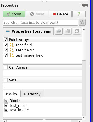
You have to choose the XdmfReader to open the file, so that Paraview may properly read the data. You will see in the Property panel, the presence of two Blocks of data, one for each grid of the dataset:

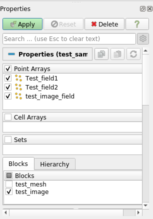
To easily visualize the Image group, untick the mesh group box in the appropriate panel, like in the image below:

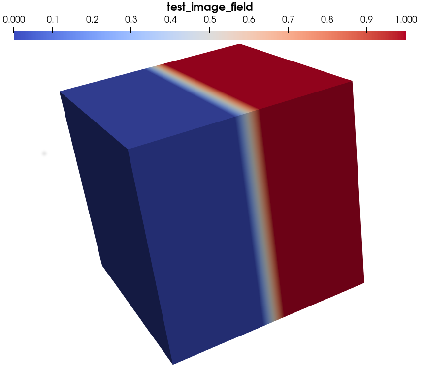
Now you can click on the Apply button: you should now see the 3D image. You can choose to plot test_image_field, which should render like this:

# Use the second code line if you want to specify the path of the paraview executable you want to use
# otherwise use the first line
#data.pause_for_visualization(Paraview=True)
#data.pause_for_visualization(Paraview=True, Paraview_path='/home/amarano/Sources/ParaView-5.9.0-RC1-MPI-Linux-Python3.8-64bit/bin/paraview')

We will print again the information on the Image Group, to focus on another aspect of the data model:

data.print_node_info('image')

 GROUP test_image
=====================
 -- Parent Group : /
 -- Group attributes :
         * description :
         * dimension : [9 9 9]
         * empty : False
         * group_type : 3DImage
         * nodes_dimension : [10 10 10]
         * nodes_dimension_xdmf : [10 10 10]
         * origin : [-1. -1. -1.]
         * spacing : [0.2 0.2 0.2]
         * xdmf_gridname : test_image
 -- Childrens : Field_index, test_image_field,
----------------

You can see that the Image group has 2 childrens, test_image_field and Field_index. Let us look at their content:

data.print_node_info('test_image_field')

 NODE: /test_image/test_image_field
====================
 -- Parent Group : test_image
 -- Node name : test_image_field
 -- test_image_field attributes :
         * empty : False
         * field_dimensionality : Scalar
         * field_type : Nodal_field
         * node_type : field_array
         * padding : None
         * parent_grid_path : /test_image
         * transpose_indices : [2, 1, 0]
         * xdmf_fieldname : test_image_field
         * xdmf_gridname : test_image

 -- content : /test_image/test_image_field (CArray(10, 10, 10)) 'image_test_image_field'
 -- Compression options for node `test_image_field`:
        complevel=0, shuffle=False, bitshuffle=False, fletcher32=False, least_significant_digit=None
 --- Chunkshape: (327, 10, 10)
 -- Node memory size :    63.867 Kb
----------------

This node is a field data item, as indicated by the node_type attribute. Those are data item designed to store the spatially organized data that are defined on grids. They will be discussed in details in section IV below.

data.print_node_info('image_Field_index')

 NODE: /test_image/Field_index
====================
 -- Parent Group : test_image
 -- Node name : Field_index
 -- Field_index attributes :
         * node_type : string array

 -- content : /test_image/Field_index (EArray(1,)) ''
 -- Compression options for node `image_Field_index`:
        complevel=0, shuffle=False, bitshuffle=False, fletcher32=False, least_significant_digit=None
 --- Chunkshape: (257,)
 -- Node memory size :    63.999 Kb
----------------

The Field Index is a String Array (see previous tutorial (section V)) that stores a list of strings that are the names of the fields stored in this Image group. You can get the list of field stored on the group by looking at this string array content:

data['image_Field_index'][0].decode('utf-8')

'image_test_image_field'

It can also be accessed easily using the get_grid_field_list method:

data.get_grid_field_list('image')

['image_test_image_field']

Now that we know what composes an Image Group, and how to visualize it, we will close the reference dataset and create one to train ourselves to create images.

del data

III - Creating Image Groups

There are three ways to create an Image group in a SampleData dataset: 1. creating an image from a data array 2. creating an image from an image object indicating its topology 3. creating an empty image

We will try all three. But first, we will once again create a temporary dataset, to try the examples of this tutorial, with verbose mode on:

data = SD(filename='tutorial_dataset', sample_name='test_sample', verbose = True, autodelete=True, overwrite_hdf5=True)

-- File "tutorial_dataset.h5" not found : file created
-- File "tutorial_dataset.xdmf" not found : file created
.... writing xdmf file : tutorial_dataset.xdmf

Minimal data model initialization....

Minimal data model initialization done

.... Storing content index in tutorial_dataset.h5:/Index attributes
.... writing xdmf file : tutorial_dataset.xdmf
.... flushing data in file tutorial_dataset.h5
File tutorial_dataset.h5 synchronized with in memory data tree

Creation an image from a data array

We will start by creating two numpy arrays that will be image fields. Their dimension will define the topology of the image. To have simple and visual examples, we will create: 1. a 2D field of dimension 51x51 representing a matrix with a circular fiber at its center, with a diameter of half the image 2. a random 3D field of dimension 50x50x50x3

We will start with the bidimensional field.

# first we need to import the Numpy package
import numpy as np

dX = 1/101
# we create a grid of coordinates to compute the distance to the center of the image
X = np.linspace(dX, 1-dX,101)
Y = np.linspace(dX, 1-dX,101)
XX, YY = np.meshgrid(X,Y)
# compute the distance function
Dist = np.sqrt(np.square(XX - 0.5) + np.square(YY - 0.5))
# creation of the 2D array: 0 indicate the matrix, 1 the fiber
field_2D = np.int16(Dist <= 0.25)

The add_image_from_field method

Now that our field is created, we can introduce the method add_image_from_field. It will create an appropriate Image group and store the data array inputed as an image field.

data.add_image_from_field(field_array=field_2D, fieldname='test_2D_field', imagename='first_2D_image',
                         indexname='image2D', location='/',
                         description="Test image group created from a bidimensional Numpy array.")

 (get_attribute) neither indexname nor node_path passed, node return aborted

Creating Group group `first_2D_image` in file tutorial_dataset.h5 at /
Updating xdmf tree...

Adding field `test_2D_field` into Grid `/first_2D_image`

Adding array `test_2D_field` into Group `/first_2D_image`

(get_node) ERROR : Node name does not fit any hdf5 path nor index name.

Adding String Array `Field_index` into Group `/first_2D_image`

The verbose mode of the class instructed us that the image group has been created, along with a field/array object. You see that the method accepts similar arguments that the ones studied in the previous tutorial. Note that here the indexname argument is for the image group indexname, the field indexname being constructed from the field_name argument (see below). To add another name to the field, you may use the add_alias method. Note also that the description argument here allows to set the description attribute of the created image group.

We will now print the content of our dataset to see the results of the image group creation:

data.print_dataset_content()

Printing dataset content with max depth 3

****** DATA SET CONTENT ******
 -- File: tutorial_dataset.h5
 -- Size:     3.469 Kb
 -- Data Model Class: SampleData

 GROUP /
=====================
 -- Parent Group : /
 -- Group attributes :
         * description :
         * sample_name : test_sample
 -- Childrens : Index, first_2D_image,
----------------
************************************************


 GROUP first_2D_image
=====================
 -- Parent Group : /
 -- Group attributes :
         * description : Test image group created from a bidimensional Numpy array.
         * dimension : [101 101]
         * empty : False
         * group_type : 2DImage
         * nodes_dimension : [102 102]
         * nodes_dimension_xdmf : [102 102]
         * origin : [0. 0.]
         * spacing : [1. 1.]
         * xdmf_gridname : first_2D_image
 -- Childrens : test_2D_field, Field_index,
----------------
****** Group /first_2D_image CONTENT ******

 NODE: /first_2D_image/Field_index
====================
 -- Parent Group : first_2D_image
 -- Node name : Field_index
 -- Field_index attributes :
         * empty : True
         * node_type : string_array

 -- content : /first_2D_image/Field_index (EArray(1,)) ''
 -- Compression options for node `/first_2D_image/Field_index`:
        complevel=0, shuffle=False, bitshuffle=False, fletcher32=False, least_significant_digit=None
 --- Chunkshape: (257,)
 -- Node memory size :    63.999 Kb
----------------

 NODE: /first_2D_image/test_2D_field
====================
 -- Parent Group : first_2D_image
 -- Node name : test_2D_field
 -- test_2D_field attributes :
         * empty : False
         * field_dimensionality : Scalar
         * field_type : Element_field
         * node_type : field_array
         * padding : None
         * parent_grid_path : /first_2D_image
         * transpose_indices : [1, 0]
         * xdmf_fieldname : test_2D_field
         * xdmf_gridname : first_2D_image

 -- content : /first_2D_image/test_2D_field (CArray(101, 101)) 'image2D_test_2D_field'
 -- Compression options for node `/first_2D_image/test_2D_field`:
        complevel=0, shuffle=False, bitshuffle=False, fletcher32=False, least_significant_digit=None
 --- Chunkshape: (324, 101)
 -- Node memory size :    63.914 Kb
----------------


************************************************

Reading its attributes, we can observe that a 2DImage group has been created, with a dimension of 51x51 pixels, in accordance with the inputed numpy array shape. We also can see that two childrens have been created for this group, a Field_index children, and a test_2D_field containing our data array (51x51 Carray).

If we look at the dataset Index, we obtain:

data.print_index()

Dataset Content Index :
------------------------:
index printed with max depth `3` and under local root `/`

         Name : image2D                                   H5_Path : /first_2D_image
         Name : image2D_test_2D_field                     H5_Path : /first_2D_image/test_2D_field
         Name : image2D_Field_index                       H5_Path : /first_2D_image/Field_index

You can see that the indexnames of the field and Field Index data items have been automatically constructed, following the rule:

indexname = grid_name + '_' + node_name.

We will look now at the other topology attributes of our Image group:

data.print_node_attributes('image2D')

 -- first_2D_image attributes :
         * description : Test image group created from a bidimensional Numpy array.
         * dimension : [101 101]
         * empty : False
         * group_type : 2DImage
         * nodes_dimension : [102 102]
         * nodes_dimension_xdmf : [102 102]
         * origin : [0. 0.]
         * spacing : [1. 1.]
         * xdmf_gridname : first_2D_image

You can observe that the origin and spacing attributes have been set to their default value ([0.,0.] and [1.,1.]), as they have not been specified in add_image_from_field arguments. We will see how to modify values for these attributes in the next subsection of this tutorial.

Create an image with specific pixel/voxel size and origin

We will now use again the image group add method to recreate our image, this time specifying the value of the grid spacing and origin:

data.add_image_from_field(field_array=field_2D, fieldname='test_2D_field', imagename='first_2D_image',
                         indexname='image2D', location='/', replace=True,
                         description="Test image group created from a bidimensional Numpy array.",
                         origin=[0.,10.], spacing=[2.,2.])

Removing group first_2D_image to replace it by new one.

Removing  node /first_2D_image in content index....

Removing  node /first_2D_image/test_2D_field in content index....


item image2D_test_2D_field : /first_2D_image/test_2D_field removed from context index dictionary
.... Storing content index in tutorial_dataset.h5:/Index attributes
.... writing xdmf file : tutorial_dataset.xdmf
.... flushing data in file tutorial_dataset.h5
File tutorial_dataset.h5 synchronized with in memory data tree

Node <closed tables.carray.CArray at 0x7ff2a31adc30> sucessfully removed

Removing  node /first_2D_image/Field_index in content index....


item image2D_Field_index : /first_2D_image/Field_index removed from context index dictionary
.... Storing content index in tutorial_dataset.h5:/Index attributes
.... writing xdmf file : tutorial_dataset.xdmf
.... flushing data in file tutorial_dataset.h5
File tutorial_dataset.h5 synchronized with in memory data tree

Node <closed tables.earray.EArray at 0x7ff2a31adcd0> sucessfully removed

item image2D : /first_2D_image removed from context index dictionary
.... Storing content index in tutorial_dataset.h5:/Index attributes
.... writing xdmf file : tutorial_dataset.xdmf
.... flushing data in file tutorial_dataset.h5
File tutorial_dataset.h5 synchronized with in memory data tree

Node /first_2D_image sucessfully removed

Creating Group group `first_2D_image` in file tutorial_dataset.h5 at /
Updating xdmf tree...

Adding field `test_2D_field` into Grid `/first_2D_image`

Adding array `test_2D_field` into Group `/first_2D_image`

(get_node) ERROR : Node name does not fit any hdf5 path nor index name.

Adding String Array `Field_index` into Group `/first_2D_image`

Note that we had to set the ``replace`` argument to ``True`` to be able to overwrite our Image group in the dataset.

data.print_node_attributes('image2D')

 -- first_2D_image attributes :
         * description : Test image group created from a bidimensional Numpy array.
         * dimension : [101 101]
         * empty : False
         * group_type : 2DImage
         * nodes_dimension : [102 102]
         * nodes_dimension_xdmf : [102 102]
         * origin : [ 0. 10.]
         * spacing : [2. 2.]
         * xdmf_gridname : first_2D_image

This time, the origin and spacing attributes have been set accordingly to our choice. Have they also been set in the XDMF file ?

data.print_xdmf()

<Xdmf xmlns:xi="http://www.w3.org/2003/XInclude" Version="2.2">
  <Domain>
    <Grid Name="first_2D_image" GridType="Uniform">
      <Topology TopologyType="2DCoRectMesh" Dimensions="102 102"/>
      <Geometry Type="ORIGIN_DXDY">
        <DataItem Format="XML" Dimensions="2">10.  0.</DataItem>
        <DataItem Format="XML" Dimensions="2">2. 2.</DataItem>
      </Geometry>
      <Attribute Name="test_2D_field" AttributeType="Scalar" Center="Cell">
        <DataItem Format="HDF" Dimensions="101  101" NumberType="Int" Precision="16">tutorial_dataset.h5:/first_2D_image/test_2D_field</DataItem>
      </Attribute>
    </Grid>
  </Domain>
</Xdmf>

The answer is yes !

You may note that in the XDMF file, the grid origin is stored as \([10, 0]\) and not \([0, 10]\), as it was inputed. This is due to the inverse interpretation of coordinate order by Paraview when visually rendering data. Hence, the values of the various data items in the XDMF file are written with an inverse coordinate order.

To modify an image spacing or origin, you can use the set_voxel_size and set_origin methods:

data.set_voxel_size(image_group='image2D', voxel_size=np.array([4.,4.]))
data.set_origin(image_group='image2D', origin=np.array([10.,0.]))
data.print_node_attributes('image2D')
data.print_xdmf()

.... Storing content index in tutorial_dataset.h5:/Index attributes
.... writing xdmf file : tutorial_dataset.xdmf
.... flushing data in file tutorial_dataset.h5
File tutorial_dataset.h5 synchronized with in memory data tree
.... Storing content index in tutorial_dataset.h5:/Index attributes
.... writing xdmf file : tutorial_dataset.xdmf
.... flushing data in file tutorial_dataset.h5
File tutorial_dataset.h5 synchronized with in memory data tree
 -- first_2D_image attributes :
         * description : Test image group created from a bidimensional Numpy array.
         * dimension : [101 101]
         * empty : False
         * group_type : 2DImage
         * nodes_dimension : [102 102]
         * nodes_dimension_xdmf : [102 102]
         * origin : [10.  0.]
         * spacing : [4. 4.]
         * xdmf_gridname : first_2D_image

<Xdmf xmlns:xi="http://www.w3.org/2003/XInclude" Version="2.2">
  <Domain>
    <Grid Name="first_2D_image" GridType="Uniform">
      <Topology TopologyType="2DCoRectMesh" Dimensions="102 102"/>
      <Geometry Type="ORIGIN_DXDY">
        <DataItem Format="XML" Dimensions="2"> 0. 10.</DataItem>
        <DataItem Format="XML" Dimensions="2">4. 4.</DataItem>
      </Geometry>
      <Attribute Name="test_2D_field" AttributeType="Scalar" Center="Cell">
        <DataItem Format="HDF" Dimensions="101  101" NumberType="Int" Precision="16">tutorial_dataset.h5:/first_2D_image/test_2D_field</DataItem>
      </Attribute>
    </Grid>
  </Domain>
</Xdmf>

The Image Group spacing and origin have indeed been modified in the group attributes, and the XDMF file.

You can use those methods to translate and dilate your image group in the visualization rendered by Paraview, which can be usefull to avoid grid superposition if you want to visualize them in the same RenderView, or, on the contrary, to force visual superposition of grids that had not the same position/scale when added to the dataset.

Creating images from pixel wise or nodal value defined fields

By using the is_elemField argument of add_image_from_field, we can change this standard behavior. By setting it to False, the method will consider the inputed array as a nodal value field: each value will be associated with a node of the image regular grid. We can test it by creating another image group from the same array:

data.add_image_from_field(field_array=field_2D, fieldname='field_nodes_2D', imagename='image_2D_bis',
                         indexname='image2D_bis', location='/',
                         description="Test image group created from a bidimensional Numpy array.",
                         origin=[0.,10.], spacing=[2.,2.], is_elemField=False)

 (get_attribute) neither indexname nor node_path passed, node return aborted

Creating Group group `image_2D_bis` in file tutorial_dataset.h5 at /
Updating xdmf tree...

Adding field `field_nodes_2D` into Grid `/image_2D_bis`

Adding array `field_nodes_2D` into Group `/image_2D_bis`

(get_node) ERROR : Node name does not fit any hdf5 path nor index name.

Adding String Array `Field_index` into Group `/image_2D_bis`

data.print_xdmf()
data.print_node_info('image2D_bis')

<Xdmf xmlns:xi="http://www.w3.org/2003/XInclude" Version="2.2">
  <Domain>
    <Grid Name="first_2D_image" GridType="Uniform">
      <Topology TopologyType="2DCoRectMesh" Dimensions="102 102"/>
      <Geometry Type="ORIGIN_DXDY">
        <DataItem Format="XML" Dimensions="2"> 0. 10.</DataItem>
        <DataItem Format="XML" Dimensions="2">4. 4.</DataItem>
      </Geometry>
      <Attribute Name="test_2D_field" AttributeType="Scalar" Center="Cell">
        <DataItem Format="HDF" Dimensions="101  101" NumberType="Int" Precision="16">tutorial_dataset.h5:/first_2D_image/test_2D_field</DataItem>
      </Attribute>
    </Grid>
    <Grid Name="image_2D_bis" GridType="Uniform">
      <Topology TopologyType="2DCoRectMesh" Dimensions="101 101"/>
      <Geometry Type="ORIGIN_DXDY">
        <DataItem Format="XML" Dimensions="2">10.  0.</DataItem>
        <DataItem Format="XML" Dimensions="2">2. 2.</DataItem>
      </Geometry>
      <Attribute Name="field_nodes_2D" AttributeType="Scalar" Center="Node">
        <DataItem Format="HDF" Dimensions="101  101" NumberType="Int" Precision="16">tutorial_dataset.h5:/image_2D_bis/field_nodes_2D</DataItem>
      </Attribute>
    </Grid>
  </Domain>
</Xdmf>


 GROUP image_2D_bis
=====================
 -- Parent Group : /
 -- Group attributes :
         * description : Test image group created from a bidimensional Numpy array.
         * dimension : [100 100]
         * empty : False
         * group_type : 2DImage
         * nodes_dimension : [101 101]
         * nodes_dimension_xdmf : [101 101]
         * origin : [ 0. 10.]
         * spacing : [2. 2.]
         * xdmf_gridname : image_2D_bis
 -- Childrens : field_nodes_2D, Field_index,
----------------

As you can see, the second image group has now dimensions reduced by one for each coordinate compared to the first image group, and the associated xdmf Grid node has an attribute that is defined on Nodes.

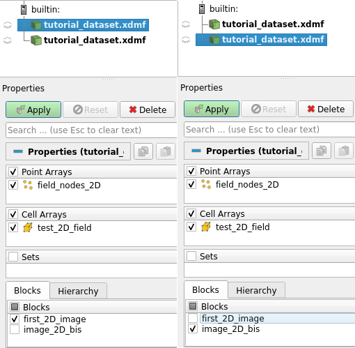
We can now visualize the fields to see what differencies does it make. Use the code of the following cell to open the dataset with Paraview. Then, you can open again the same file in Paraview, and only activate the rendering of one image group for each file, by ticking it in the property panel, as shown on the image below:

# Use the second code line if you want to specify the path of the paraview executable you want to use
# otherwise use the first line
#data.pause_for_visualization(Paraview=True)
#data.pause_for_visualization(Paraview=True, Paraview_path='path to paraview executable')

What you should see, is, for the pixel wise field, an rendering close to this:

And, for the nodal value field, you should have a rendering close to this:

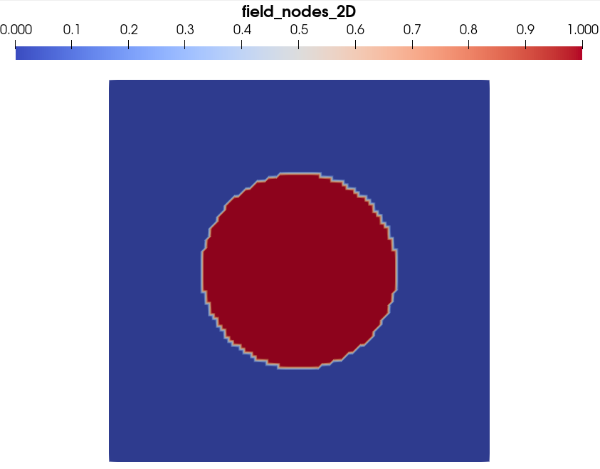
The visual difference is clear, even if it is exactly the same data array that is plotted in both cases. In the first case, with Cell centered data, Paraview interprets the data as a field constant within each element. On the contrary, in the second case, with Node centered data, Paraview interprets the data as values that the field takes at grid vertexes, and interpolate linearly field values in the pixels (the grid elements) to render the visualization. That is why the field appears continuous at the interface between the fiber and the matrix.

Creating images from scalar, vector or tensor fields

There is another argument that changes the way add_image_from_field interprets the field data array: the is_scalar argument. Its default value is True. In this case the shape of the field is interpreted as a the dimension of the image to create. In the case just above, we inputed a (101x101) field, and the method created an image group of 101x101 pixels, containing a scalar field, i.e. a field with only one value per pixel.

However, we may want to create an image from a field whose values are vector or tensors. In that case, there is an ambiguity for arrays with 3 dimensions. They can either represent a \((x,y,z)\) array, or a \((x,y,i)\) array, where \(i\) denotes the field component index.

The ``is_scalar`` argument role is to avoid this ambiguity. If it is ``True`` (default) value, a 3D array will be interpreted as a 3D :math:`(x,y,z)` scalar field, and if it is ``False``, it will be interpreted as a :math:`(x,y,i)` 2D vector or tensor field.

Time to test this feature:

# creation of a random 3D field :
field_3D = np.random.rand(50,50,3)

# creation of a 3D image group --> is_scalar set to True (default value)
data.add_image_from_field(field_array=field_3D, fieldname='field_3D', imagename='image_3D',
                          indexname='image3D', location='/',
                          description="""
                          Test 3D image group created from a tridimensional Numpy array with `is_scalar` = True.""")

# creation of a 2D image group --> is_scalar set to False
data.add_image_from_field(field_array=field_3D, fieldname='field_vect', imagename='image_2D_3',
                          indexname='image2D_3', location='/', is_scalar=False,
                          description="""
                          Test 2D image group created from a tridimensional Numpy array with `is_scalar` = False.""")

 (get_attribute) neither indexname nor node_path passed, node return aborted

Creating Group group `image_3D` in file tutorial_dataset.h5 at /
Updating xdmf tree...

Adding field `field_3D` into Grid `/image_3D`

Adding array `field_3D` into Group `/image_3D`

(get_node) ERROR : Node name does not fit any hdf5 path nor index name.

Adding String Array `Field_index` into Group `/image_3D`

 (get_attribute) neither indexname nor node_path passed, node return aborted

Creating Group group `image_2D_3` in file tutorial_dataset.h5 at /
Updating xdmf tree...

Adding field `field_vect` into Grid `/image_2D_3`

Adding array `field_vect` into Group `/image_2D_3`

(get_node) ERROR : Node name does not fit any hdf5 path nor index name.

Adding String Array `Field_index` into Group `/image_2D_3`

# Getting information on the dataset and the created image groups
print(data)
data.print_node_info('image_3D')
data.print_node_info('image_2D_3')

Dataset Content Index :
------------------------:
index printed with max depth `3` and under local root `/`

         Name : image2D                                   H5_Path : /first_2D_image
         Name : image2D_test_2D_field                     H5_Path : /first_2D_image/test_2D_field
         Name : image2D_Field_index                       H5_Path : /first_2D_image/Field_index
         Name : image2D_bis                               H5_Path : /image_2D_bis
         Name : image2D_bis_field_nodes_2D                H5_Path : /image_2D_bis/field_nodes_2D
         Name : image2D_bis_Field_index                   H5_Path : /image_2D_bis/Field_index
         Name : image3D                                   H5_Path : /image_3D
         Name : image3D_field_3D                          H5_Path : /image_3D/field_3D
         Name : image3D_Field_index                       H5_Path : /image_3D/Field_index
         Name : image2D_3                                 H5_Path : /image_2D_3
         Name : image2D_3_field_vect                      H5_Path : /image_2D_3/field_vect
         Name : image2D_3_Field_index                     H5_Path : /image_2D_3/Field_index

Printing dataset content with max depth 3
  |--GROUP first_2D_image: /first_2D_image (2DImage)
     --NODE Field_index: /first_2D_image/Field_index (string_array - empty) (   63.999 Kb)
     --NODE test_2D_field: /first_2D_image/test_2D_field (field_array) (   63.914 Kb)

  |--GROUP image_2D_3: /image_2D_3 (2DImage)
     --NODE Field_index: /image_2D_3/Field_index (string_array - empty) (   63.999 Kb)
     --NODE field_vect: /image_2D_3/field_vect (field_array) (   63.281 Kb)

  |--GROUP image_2D_bis: /image_2D_bis (2DImage)
     --NODE Field_index: /image_2D_bis/Field_index (string_array - empty) (   63.999 Kb)
     --NODE field_nodes_2D: /image_2D_bis/field_nodes_2D (field_array) (   63.914 Kb)

  |--GROUP image_3D: /image_3D (3DImage)
     --NODE Field_index: /image_3D/Field_index (string_array - empty) (   63.999 Kb)
     --NODE field_3D: /image_3D/field_3D (field_array) (   58.594 Kb)



 GROUP image_3D
=====================
 -- Parent Group : /
 -- Group attributes :
         * description :
                          Test 3D image group created from a tridimensional Numpy array with `is_scalar` = True.
         * dimension : [50 50  3]
         * empty : False
         * group_type : 3DImage
         * nodes_dimension : [51 51  4]
         * nodes_dimension_xdmf : [ 4 51 51]
         * origin : [0. 0. 0.]
         * spacing : [1. 1. 1.]
         * xdmf_gridname : image_3D
 -- Childrens : field_3D, Field_index,
----------------


 GROUP image_2D_3
=====================
 -- Parent Group : /
 -- Group attributes :
         * description :
                          Test 2D image group created from a tridimensional Numpy array with `is_scalar` = False.
         * dimension : [50 50]
         * empty : False
         * group_type : 2DImage
         * nodes_dimension : [51 51]
         * nodes_dimension_xdmf : [51 51]
         * origin : [0. 0.]
         * spacing : [1. 1.]
         * xdmf_gridname : image_2D_3
 -- Childrens : field_vect, Field_index,
----------------

# Getting information on created image fields
data.print_node_info('image3D_field_3D')
data.print_node_info('image2D_3_field_vect')

 NODE: /image_3D/field_3D
====================
 -- Parent Group : image_3D
 -- Node name : field_3D
 -- field_3D attributes :
         * empty : False
         * field_dimensionality : Scalar
         * field_type : Element_field
         * node_type : field_array
         * padding : None
         * parent_grid_path : /image_3D
         * transpose_indices : [2, 1, 0]
         * xdmf_fieldname : field_3D
         * xdmf_gridname : image_3D

 -- content : /image_3D/field_3D (CArray(3, 50, 50)) 'image3D_field_3D'
 -- Compression options for node `image3D_field_3D`:
        complevel=0, shuffle=False, bitshuffle=False, fletcher32=False, least_significant_digit=None
 --- Chunkshape: (3, 50, 50)
 -- Node memory size :    58.594 Kb
----------------



 NODE: /image_2D_3/field_vect
====================
 -- Parent Group : image_2D_3
 -- Node name : field_vect
 -- field_vect attributes :
         * empty : False
         * field_dimensionality : Vector
         * field_type : Element_field
         * node_type : field_array
         * padding : None
         * parent_grid_path : /image_2D_3
         * transpose_indices : [1, 0, 2]
         * xdmf_fieldname : field_vect
         * xdmf_gridname : image_2D_3

 -- content : /image_2D_3/field_vect (CArray(50, 50, 3)) 'image2D_3_field_vect'
 -- Compression options for node `image2D_3_field_vect`:
        complevel=0, shuffle=False, bitshuffle=False, fletcher32=False, least_significant_digit=None
 --- Chunkshape: (54, 50, 3)
 -- Node memory size :    63.281 Kb
----------------

If you look at the two created image groups, you see indeed that one has been created as a 3DImage group (with is_scalar=True), and one as a 2DImage Group (with is_scalar=False). Moreover, the field_dimensionality attribute of the two created image fields state clearly that the field of the 3D image is a scalar field, whereas the other one is a vector field.

We can now visualize them:

# Use the second code line if you want to specify the path of the paraview executable you want to use
# otherwise use the first line
#data.pause_for_visualization(Paraview=True)
#data.pause_for_visualization(Paraview=True, Paraview_path='path to paraview executable')

The rendering of the 3D image group with Paraview, containing a random 3D scalar field, should look the image below:

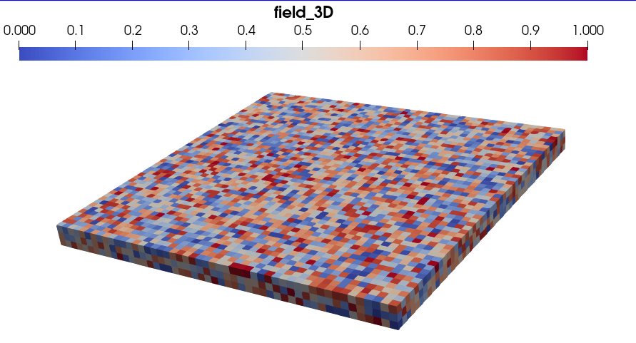
To obtain the rendering above, we only activated the rendering of the ``image_3D`` block in Paraview’s window Property Panel, and plotted it with the Surface renderer.

The rendering of the 2D image group with Paraview, containing a random 2D vector field, should look the this:

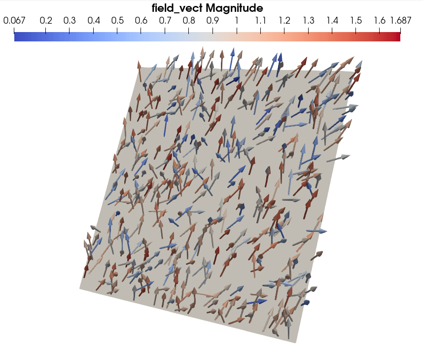
To obtain the rendering above, we only activated the rendering of the ``image_2D_3`` block in Paraview’s window Property Panel, added a Glyph filter in Arrow mode (that is how to plot vector field with Paraview) and colored the arrows with the vector field magnitude. We also bounded the maximum number of plotted arrows to 500.

We will stress again that here, those two very different visual rendering where obtained by creating two image groups with stricly the same input field data array. This illustrate the formatting possibilities offered by the SampleData class, but also highlight the need to be familiar with them, and to clearly specify in what form the data must be stored, to avoid unwanted behaviors.

Note that you can see in the attributes of the 3D image group the dimension transposition between \(X\) and \(Z\) coordinates, mentioned in section II, when comparing the values of attributes nodes_dimension and nodes_dimension_xdmf.

Note that we could have executed the same lines with an array of shape \((50,50,6)\) or \((50,50,9)\). The resulting 2D image would have in those cases supported a symetric tensor or tensor field.

This closes the presentation of the first and more straightforward way to create an Image group in a SampleData dataset.

Creating images from image objects

The second way to create Image groups, requires the creation of an image object. To handle grids, the SampleData class relies on the BasicTools Python package, developed by the industrial group Safran. This package offers some classes to represent meshes, and in particular rectilinear meshes, i.e. regular grids. What whe refer to as an image object, is in fact a BasicTools rectilinear mesh object. Let us see how it works with an example.

First, we need to import the rectilinear mesh class from Basictools, that should be accessible in your python environment as it is a SampleData dependence:

from BasicTools.Containers.ConstantRectilinearMesh import ConstantRectilinearMesh

Then, we will create our image object as an instance of this class. For that, we need to set its dimenion (2D or 3D) image. For this example, we will try to recreate the 3D image with the random scalar field:

image_object = ConstantRectilinearMesh(dim=3)
print(type(image_object))

<class 'BasicTools.Containers.ConstantRectilinearMesh.ConstantRectilinearMesh'>

We can now set the topology of the image, by using the following methods:

image_object.SetDimensions((50,50,3))
image_object.SetOrigin([0.,0.,0.])
image_object.SetSpacing([1.,1.,1.])

Finally, image objects have two attributes that are dictionaries, the elemFields and the nodeFields, that allow to add fields to the image. Of course, these fields should have dimensions that match the image object dimensions. We will then add our random 3D array as a field of this image:

image_object.elemFields['im_object_field'] = field_3D

We can print our image object to get information on it:

print(image_object)

ConstantRectilinearMesh
  Number of Nodes    : 7500
    Tags :
  Number of Elements : 4802
  dimensions         : [50 50  3]
  origin             : [0. 0. 0.]
  spacing            : [1. 1. 1.]
    ConstantRectilinearElementContainer,   Type : (hex8,4802),   Tags :

  Node Tags          : []
  Cell Tags          : []
  elemFields         : ['im_object_field']

You can see that it has an attribute that is an Element container, that has 4802 elements of type hex8, i.e. linear hexaedra, which is consistent with a grid of voxels.

Now we can add the image into the dataset with the add_image method. Its arguments are exactly the same as those of the add_image_from_field method, without the field_array, fieldname, is_scalar, elemField arguments:

data.add_image(image_object, imagename='image_from_object', indexname='imageO', location='/',
               description="""Test 3D image group created from an image object.""")

 (get_attribute) neither indexname nor node_path passed, node return aborted

Creating Group group `image_from_object` in file tutorial_dataset.h5 at /
Updating xdmf tree...

Adding field `im_object_field` into Grid `/image_from_object`

Adding array `im_object_field` into Group `/image_from_object`

(get_node) ERROR : Node name does not fit any hdf5 path nor index name.

Adding String Array `Field_index` into Group `/image_from_object`

<BasicTools.Containers.ConstantRectilinearMesh.ConstantRectilinearMesh at 0x7ff2a30ef050>

data.print_node_info('imageO')

 GROUP image_from_object
=====================
 -- Parent Group : /
 -- Group attributes :
         * description : Test 3D image group created from an image object.
         * dimension : [49 49  2]
         * empty : False
         * group_type : 3DImage
         * nodes_dimension : [50 50  3]
         * nodes_dimension_xdmf : [ 3 50 50]
         * origin : [0. 0. 0.]
         * spacing : [1. 1. 1.]
         * xdmf_gridname : image_from_object
 -- Childrens : im_object_field, Field_index,
----------------

The image group has been created. Though, you can see that the dimension we indicated, actually prescribed the image nodes_dimension. Hence, remember that the ``SetDimensions`` method of image objects set the dimension of the node grid. The pixel/voxel grid has the same dimensions minus one along each direction.

As a result, we should expect here that the field loaded into the image object has been added to the image group as a nodal field. We can verify it by printing its attributes:

data.print_node_attributes('imageO_im_object_field')

 -- im_object_field attributes :
         * empty : False
         * field_dimensionality : Scalar
         * field_type : Nodal_field
         * node_type : field_array
         * padding : None
         * parent_grid_path : /image_from_object
         * transpose_indices : [2, 1, 0]
         * xdmf_fieldname : im_object_field
         * xdmf_gridname : image_from_object

which, confirms our guess.

All the variations linked to the fields presented in above can still be achieved with this way of adding images in the datasets. For instance, if you passed to SetDimension the tuple \((N_x,N_y,N_z)\), to add a nodal vector field to your image group add a \((N_x,N_y,N_z,3)\) array to the image object elemFields list.

Creating empty images

SampleData also offers the possibility to create empty image objects. To do this, you proceed also with the add_image method, but without providing any image object:

data.add_image(imagename='image_empty', indexname='imageE', location='/',
               description="""Test empty image group.""")

 (get_attribute) neither indexname nor node_path passed, node return aborted

Creating Group group `image_empty` in file tutorial_dataset.h5 at /

data.print_node_info('imageE')

 GROUP image_empty
=====================
 -- Parent Group : /
 -- Group attributes :
         * empty : True
         * group_type : emptyImage
 -- Childrens :
----------------

Like empty data arrays presented in the tutorial 2 (section IV), empty images are used to create the internal organization of your dataset without having to add any data to it. It allows for instance to preempt some data item names, indexnames, and to already add metadata. When you have data to add, you can then create an image group with the same name/location, the empty image will be replace by an actual image group, but all metadata that was added to it before will be preserved.

To test this, we start by adding metadata to our empty image group:

data.add_attributes({'tutorial_file':'3_SampleData_Image_groups.ipynb', 'tutorial_section':'III'}, 'imageE')
data.print_node_attributes('imageE')

 -- image_empty attributes :
         * empty : True
         * group_type : emptyImage
         * tutorial_file : 3_SampleData_Image_groups.ipynb
         * tutorial_section : III

Now we will overwrite the empty image group by creating a 3D image group (same as in last subsection). In this case we do not need to set the replace argument to True.

# first, we will change the name of the field stored in the image object ti avoid duplicates in the dataset
data.add_image(image_object, imagename='image_empty', indexname='imageE', location='/',
               description="""Test empty image group overwritten with actual data.""")
data.print_node_info('imageE')

item imageE : /image_empty removed from context index dictionary
Updating xdmf tree...

Adding field `im_object_field` into Grid `/image_empty`

Adding array `im_object_field` into Group `/image_empty`

(get_node) ERROR : Node name does not fit any hdf5 path nor index name.

Adding String Array `Field_index` into Group `/image_empty`

 GROUP image_empty
=====================
 -- Parent Group : /
 -- Group attributes :
         * description : Test empty image group overwritten with actual data.
         * dimension : [49 49  2]
         * empty : False
         * group_type : 3DImage
         * nodes_dimension : [50 50  3]
         * nodes_dimension_xdmf : [ 3 50 50]
         * origin : [0. 0. 0.]
         * spacing : [1. 1. 1.]
         * tutorial_file : 3_SampleData_Image_groups.ipynb
         * tutorial_section : III
         * xdmf_gridname : image_empty
 -- Childrens : im_object_field, Field_index,
----------------

The creation of the image group with actual data has indeed preserved the attributes attached to the former empty node.

Now, you know all about the three methods to create image groups in SampleData datasets.

IV - Image Fields data model

In this new section, we will now focus on the definition of image fields data items. Fields are data arrays with additional metadata allowing to interpret them as spatially organized data. For the SampleData class, these metadata main roles are to ensure that: 1. the correspondance between dimensions of the field array values and their physical meaning is preserved from the user perspective 2. that the fields visualization with Paraview through the XDMF format properly renders the geometry and dimensionality of fields values

To that, some conventions have been defined.

SampleData Image fields conventions

Image grids coordinates

Two grids are associated to Image Groups:

• a grid of pixel/voxel centers, of dimensions \((N_x, N_y)\) or \((N_x, N_y, N_z)\), that can be seen as a set of points indentified by a doublet/triplet index:

  • \(P^c (i,j) = (x^c_i,y^c_j)\) (2D images)

  • $ P^c (i,j,k) = (x:sup:c_i,yc_j,z^c_k)$ (3D images)

• a grid of nodes (pixel/voxel vertexes), of dimensions \((N_x+1, N_y+1)\) or \((N_x+1, N_y+1, N_z+1)\), similarly defined:

  • \(P^n (i,j) = (x^n_i, y^n_ j)\) (2D images)

  • \(P^n (i,j,k) = (x^n_i, y^n_ j, z^n_ k)\) (3D images)

with \(x^c,y^c\) and \(z^c\) representing the coordinates or pixel/voxel centers and \(x^n,y^n\) and \(z^n\) representing the coordinates or pixel/voxel centers.

Fields array possible shapes

You can add numpy arrays as fields to SampleData image groups. This array specifies the data of the field for each point of one of those two grids. It must have at least as many dimensions as the grid. Fields array are only allowed to have one more dimension that the grid they are defined on, and their first dimension sizes must comply with the grid dimensions. This implies that field arrays can only have 8 different types of shapes:

1. 2D grids:

   1. \(F(i,j) \longrightarrow\) size \((N_x,N_y)\)

   2. \(F(i,j,c) \longrightarrow\) size \((N_x,N_y,N_c)\)

   3. \(F(i,j) \longrightarrow\) size \((N_x+1,N_y+1)\)

   4. \(F(i,j,c) \longrightarrow\) size \((N_x+1,N_y+1,N_c+1)\)

2. 3D grids:

   1. \(F(i,j,k) \longrightarrow\) size \((N_x,N_y, N_z)\)

   2. \(F(i,j,k,c) \longrightarrow\) size \((N_x,N_y, N_c)\)

   3. \(F(i,j,k) \longrightarrow\) size \((N_x +1,N_y +1, N_z +1)\)

   4. \(F(i,j,k,c) \longrightarrow\) size \((N_x +1,N_y +1, N_c +1)\)

Field dimensionality

The size of the last dimension of the array determines the number of field components \(N_c\), which defines the field dimensionality. If the array has no supplementary dimension with respect to the grid, i.e. no \(c\) index, then \(N_c=1\).

SampleData will interpret the field dimensionality (scalar, vector, or tensor) depending on the grid topology and the array shape. All possibilities are listed hereafter: * \(N_c=1\): scalar field * \(N_c=3\): vector field * \(N_c=6\): symetric tensor field (2nd order tensor) * \(N_c=9\): tensor field (2nd order tensor)

The dimensionality of the field has the following implications: * XDMF: the dimensionality of the field is one of the metadata stored in the XDMF file, for Fields (Attribute nodes) * visualization: as it is stored in the XDMF file, Paraview can correctly interpret the fields according to their dimensionality. Il allows to plot separately each field component, and the field norm (magnitude). It also allows to use the Paraview Glyph filter to plot vector fields with arrows * indexing: The order of the value in the last dimension for non-scalar fields correspond to a specific order of the field components, according to a specific convention. These conventions will be detailed in the next subsection. * compression: Specific lossy compression options exist for fields. See dedicated tutorial. * interface with external tools: when interfacing SampleData with external softwares, such as numerical simulation tools, it is very practical to have fields with appropriate dimensionality accounted for (for instance to use a displacement or temperature gradient vector field stored in a SampleData dataset as input for a finite element simulation).

Field components indexing

We will now review the conventions for the correspondance between field data arrays indexing and field components, hence field arrays whose indexing is \(F[i,j,c]\) or \(F[i,j,k,c]\). To detail the convention, we will omit the spatial indexes \(i,j\) or \(k\) and only consider the last dimension of the field: \(F[i,j,k,c] = F[c]\). We additionally use the subscript notation \(F[c] = F_c\).

The indexing conventions are:

• For vector fields (3 components), the convention is \([F_0,F_1,F_2] = [F_x,F_y,F_z]\)

• For symetric tensor fields (2nd order, 6 components), the convention is \([F_0,F_1,F_2,F_3,F_4,F_5] = [F_{xx},F_{yy},F_{zz},F_{xy},F_{yz},F_{zx}]\)

• For tensor fields (2nd order, 9 components), the convention is \([F_0,F_1,F_2,F_3,F_4,F_5,F_6,F_7,F_8] = [F_{xx},F_{yy},F_{zz},F_{xy},F_{yz},F_{zx},F_{yx},F_{zy},F_{xz}]\)

For the first indices, the convention is \(F[i,j,c] = F(x_i,y_i)[c]\) (2D) and \(F[i,j,k,c] = F(x_i,y_j,z_k)[c]\) (3D)

Here are a few examples to illustrate those conventions:

• \(F[10,23]\) can only be interpreted as:

  • the field value at the grid point \((x_{10},y_{23})\)

• \(F[10,23,2]\) can be interpreted as:

  • if \(F\) is a scalar field: the field value at the grid point \((x_{10},y_{23}, z_2)\)

  • if \(F\) is a vector field: the \(F_z\) component value at the grid point \((x_{10},y_{23})\)

  • if \(F\) is a tensor field: the \(F_{zz}\) component value at the grid point \((x_{10},y_{23})\)

• \(F[10,23,7]\) can be interpreted as:

  • if \(F\) is a scalar field: the field value at the grid point \((x_{10},y_{23}, z_{7})\)

  • if \(F\) is a tensor field (non-symetric): the \(F_{zy}\) component value at the grid point \((x_{10},y_{23})\)

• \(F[10,23,24,1]\) can be interpreted as:

  • if \(F\) is a vector field: the \(F_y\) component value at the grid point \((x_{10},y_{23},z_{24})\)

  • if \(F\) is a tensor field: the \(F_{yy}\) component value at the grid point \((x_{10},y_{23},z_{24})\)

• \(F[10,23,24,5]\) can only be interpreted as:

  • the \(F_{zy}\) component value (tensor field) at the grid point \((x_{10},y_{23},z_{24})\)

Warning

Field components (example: \(x,y,xx,zy\)…) are assumed to be defined in the same frame as the grid. However, that cannot be ensured simply by providing a data array. Hence, the user must ensure to have this coincidence between the grid and the data. It is not mandatory, but not respecting this implicit convention may lead to confusions and geometrical misinterpretation of the data by other users or software. If you want to do it, a good idea would be to add attributes to the field to specify and explain the nature of the field components.

Field indices in-memory transposition

The indexing convention presented in the last subsection apply to data array that we add to Image groups as fields, and to data array that are retrieved from dataset Image group fields. However, you will see below that the fields are not stored in the HDF5 file with the same ordering. In practice, two transpositions are applied to the data arrays before loading them into the dataset, to ensure proper visualization with the Paraview software. There are two reasons for it, linked to Paraview indexing conventions:

1. Paraview convention for spatial indices is inverse to *SampleData* condition:

   • 2D: the dimensions \(0\) and \(1\) must be inverted: \(F[i,j,...] \longrightarrow F[j,i,...]\)

   • 3D: the dimensions \(0\) and \(2\) must be inverted: \(F[i,j,k,...] \longrightarrow F[k,j,i,...]\)

For these reason, fields are stored with indices transposition in SampleData datasets so that their visualization with Paraview yield a rendering that is consistent with the ordering convention presented in the previous subsection. These transposition are automatically handled, as well as the back transposition when a field is retrieved, as you will see in the last section of this tutorial.

An attribute ``transpose_indices`` is added to field data items. Its values represent the order in the first columns of the original array are stored in memory (see examples below).

2. Paraview component order convention is different from *SampleData* condition for tensors. The convention in Paraview is:

   • \([F_0,F_1,F_2,F_3,F_4,F_5] = [F_{xx},F_{xy},F_{xz},F_{yy},F_{yz},F_{zz}]\) for symetric tensors

   • \([F_0,F_1,F_2,F_3,F_4,F_5,F_6,F_7,F_8] = [F_{xx},F_{xy},F_{xz},F_{yx},F_{yy},F_{yz},F_{zx},F_{zy},F_{zz}]\) for non symetric tensors

For these reason, fields are stored with indices transposition in SampleData datasets so that their visualization with Paraview yield a rendering that is consistent with the ordering convention presented in the previous subsection. These transposition are automatically handled, as well as the back transposition when a field is retrieved, as you will see in the last section of this tutorial.

An attribute ``transpose_components`` is added to field data items. Its values represent the order in which components or the original array are stored in memory (see examples below).

Note

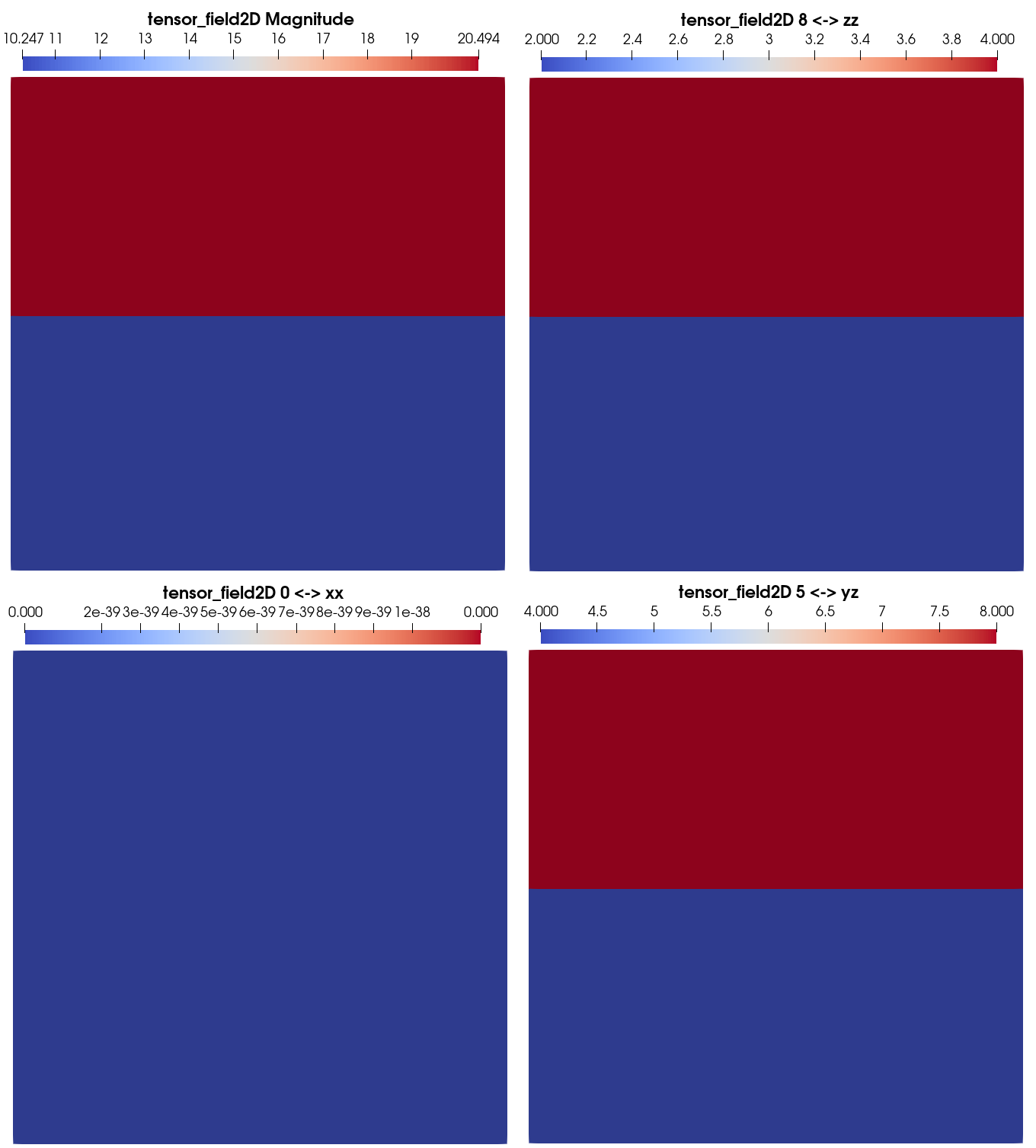
When visualizing a field in paraview, you may choose which component (including field magnitude) you are plotting in the box (highlighted in red in the image below) located in between the boxes for the choice of the visualization mode (Surface in the image below) and the data item choice (tensor_field2D in the image below).

In this box, you will have to choose between 9 (0 to 8) components, even for symetric tensors. In the later case, the corresponding equal components (1 and 3: \(xy\)&\(yx\), 2 and 6: \(xz\)&\(zx\), 5 and 7: \(yz\)&\(zy\)) will yield the same visualization.

Field type

In addition to their dimensionality, Image Fields data items also have a field type. You already encountered the two field types that can be supported by image groups in section III:

• element field:

  • described by an array of values defined at pixel/voxel centers \(P^c\) (dimension \((N_x,N_y,N_c)\) or \((N_x,N_y,N_z,N_c)\) )

  • visualization: a pixel/voxel wise constant fields

• nodal field:

  • described by an array of values defined at grid nodes (pixel/voxel vertexes) \(P^n\) (dimension \((N_x+1,N_y+1, N_c)\) or \((N_x+1,N_y+1,N_z+1,N_c)\) )

  • visualization: field linearly interpolated within each pixel/voxel from values at nodes

This feature is stored in the field data item attribute field_type (see examples above in section III).

Warning

Paraview seems to be unable to read non-scalar nodal fields XDMF Attributes for nodal regular grids. However, element vector or tensor fields can be visualized normally.

Field attributes

For each field, the value of all features presented above are stored as attributes. Let us see an example:

data.print_index()

Dataset Content Index :
------------------------:
index printed with max depth `3` and under local root `/`

         Name : image2D                                   H5_Path : /first_2D_image
         Name : image2D_test_2D_field                     H5_Path : /first_2D_image/test_2D_field
         Name : image2D_Field_index                       H5_Path : /first_2D_image/Field_index
         Name : image2D_bis                               H5_Path : /image_2D_bis
         Name : image2D_bis_field_nodes_2D                H5_Path : /image_2D_bis/field_nodes_2D
         Name : image2D_bis_Field_index                   H5_Path : /image_2D_bis/Field_index
         Name : image3D                                   H5_Path : /image_3D
         Name : image3D_field_3D                          H5_Path : /image_3D/field_3D
         Name : image3D_Field_index                       H5_Path : /image_3D/Field_index
         Name : image2D_3                                 H5_Path : /image_2D_3
         Name : image2D_3_field_vect                      H5_Path : /image_2D_3/field_vect
         Name : image2D_3_Field_index                     H5_Path : /image_2D_3/Field_index
         Name : imageO                                    H5_Path : /image_from_object
         Name : imageO_im_object_field                    H5_Path : /image_from_object/im_object_field
         Name : imageO_Field_index                        H5_Path : /image_from_object/Field_index
         Name : imageE                                    H5_Path : /image_empty
         Name : imageE_im_object_field                    H5_Path : /image_empty/im_object_field
         Name : imageE_Field_index                        H5_Path : /image_empty/Field_index

data.print_node_info('image2D_3_field_vect')

 NODE: /image_2D_3/field_vect
====================
 -- Parent Group : image_2D_3
 -- Node name : field_vect
 -- field_vect attributes :
         * empty : False
         * field_dimensionality : Vector
         * field_type : Element_field
         * node_type : field_array
         * padding : None
         * parent_grid_path : /image_2D_3
         * transpose_indices : [1, 0, 2]
         * xdmf_fieldname : field_vect
         * xdmf_gridname : image_2D_3

 -- content : /image_2D_3/field_vect (CArray(50, 50, 3)) 'image2D_3_field_vect'
 -- Compression options for node `image2D_3_field_vect`:
        complevel=0, shuffle=False, bitshuffle=False, fletcher32=False, least_significant_digit=None
 --- Chunkshape: (54, 50, 3)
 -- Node memory size :    63.281 Kb
----------------

The attribute printed above inform us on the field data item features. The field_dimensionality attribute indicates that the field is a vector field. Has its data array has a dimension of 3 (see the content line in the output), it is a scalar field of a 2D image. The field_type attribute indicates that the field is defined at pixel centers.

The transpose_indices show that the first and second column of the original inputed array have been inverted in memory (inversion of \(X\) and \(Y\) direction between SampleData and Paraview conventions).

The parent_grid_path and xdmf_gridname attribute provides the path of the Image Group and the XDMF Grid Node name to which this field belongs. The xdmf_fieldname provides the name of the XDMF Attribute Node associated to the field. The padding attribute is of no use for Image fields. It will be presented in the next tutorial for mesh fields.

V - Adding Fields to Image Groups

Now that we know all elements that compose and define a field data item in a SampleData dataset, we will see how to create fields. As for other creation tasks, the SampleData class provides a method to do it with an explicit name: the add_field method. It is very similar to the add_data_array method, with two main additions presented below.

Adding a field to a grid

To add a field to a grid from a numpy array, you just have to call add_field like you would have called add_data_array, with an additional argument gridname, that indicates the grid group to which you want to add the field. In the case of the present tutorial, we can hence provide the Name, Indexname, Path or Alias of an image group to add a field.

The analysis of the field dimensionality, nature and required transpositions is automatically handled by the class.

We will try to add a symetric tensor element field to the first 2D image that we have created, at the beginning of section III. Let us recall the image group features:

data.print_node_info('image2D')

 GROUP first_2D_image
=====================
 -- Parent Group : /
 -- Group attributes :
         * description : Test image group created from a bidimensional Numpy array.
         * dimension : [101 101]
         * empty : False
         * group_type : 2DImage
         * nodes_dimension : [102 102]
         * nodes_dimension_xdmf : [102 102]
         * origin : [10.  0.]
         * spacing : [4. 4.]
         * xdmf_gridname : first_2D_image
 -- Childrens : test_2D_field, Field_index,
----------------

The image has a nodes_dimension of 102x102. We can retrieve this attribute to presscribe the shape of the array that we have to create. As we want to create a symetric tensor field, we also need to add a last dimension of size 6.

We will create a very simple field, whose values are defined by \(F(i,j,c) = c\) for \(y <= 51\) and \(F(i,j,c) = 2c\) for \(y > 51\):

# first we get the image nodal grid dimensions
dim = data.get_attribute('dimension','image2D')

# then, we create a field of 0 with the right dimensions
Nc = 6
tensor_field = np.zeros(shape=(dim[0],dim[1],Nc))

# finally we set the values of our tensor field
for c in range(Nc):
    tensor_field[:,:52,c] = c
    tensor_field[:,52:,c] = 2*c

print(tensor_field)

[[[ 0.  1.  2.  3.  4.  5.]
  [ 0.  1.  2.  3.  4.  5.]
  [ 0.  1.  2.  3.  4.  5.]
  ...
  [ 0.  2.  4.  6.  8. 10.]
  [ 0.  2.  4.  6.  8. 10.]
  [ 0.  2.  4.  6.  8. 10.]]

 [[ 0.  1.  2.  3.  4.  5.]
  [ 0.  1.  2.  3.  4.  5.]
  [ 0.  1.  2.  3.  4.  5.]
  ...
  [ 0.  2.  4.  6.  8. 10.]
  [ 0.  2.  4.  6.  8. 10.]
  [ 0.  2.  4.  6.  8. 10.]]

 [[ 0.  1.  2.  3.  4.  5.]
  [ 0.  1.  2.  3.  4.  5.]
  [ 0.  1.  2.  3.  4.  5.]
  ...
  [ 0.  2.  4.  6.  8. 10.]
  [ 0.  2.  4.  6.  8. 10.]
  [ 0.  2.  4.  6.  8. 10.]]

 ...

 [[ 0.  1.  2.  3.  4.  5.]
  [ 0.  1.  2.  3.  4.  5.]
  [ 0.  1.  2.  3.  4.  5.]
  ...
  [ 0.  2.  4.  6.  8. 10.]
  [ 0.  2.  4.  6.  8. 10.]
  [ 0.  2.  4.  6.  8. 10.]]

 [[ 0.  1.  2.  3.  4.  5.]
  [ 0.  1.  2.  3.  4.  5.]
  [ 0.  1.  2.  3.  4.  5.]
  ...
  [ 0.  2.  4.  6.  8. 10.]
  [ 0.  2.  4.  6.  8. 10.]
  [ 0.  2.  4.  6.  8. 10.]]

 [[ 0.  1.  2.  3.  4.  5.]
  [ 0.  1.  2.  3.  4.  5.]
  [ 0.  1.  2.  3.  4.  5.]
  ...
  [ 0.  2.  4.  6.  8. 10.]
  [ 0.  2.  4.  6.  8. 10.]
  [ 0.  2.  4.  6.  8. 10.]]]

# now we can add our field to the image group
data.add_field(gridname='image2D', fieldname='tensor_field2D', location='image2D', indexname='tensorF',
               array=tensor_field, replace=True)

Adding field `tensor_field2D` into Grid `image2D`

Adding array `tensor_field2D` into Group `image2D`

/first_2D_image/tensor_field2D (CArray(101, 101, 6)) 'tensorF'
  atom := Float64Atom(shape=(), dflt=0.0)
  maindim := 0
  flavor := 'numpy'
  byteorder := 'little'
  chunkshape := (13, 101, 6)

data.print_node_info('tensorF')

 NODE: /first_2D_image/tensor_field2D
====================
 -- Parent Group : first_2D_image
 -- Node name : tensor_field2D
 -- tensor_field2D attributes :
         * empty : False
         * field_dimensionality : Tensor6
         * field_type : Element_field
         * node_type : field_array
         * padding : None
         * parent_grid_path : /first_2D_image
         * transpose_components : [0, 3, 5, 1, 4, 2]
         * transpose_indices : [1, 0, 2]
         * xdmf_fieldname : tensor_field2D
         * xdmf_gridname : first_2D_image

 -- content : /first_2D_image/tensor_field2D (CArray(101, 101, 6)) 'tensorF'
 -- Compression options for node `tensorF`:
        complevel=0, shuffle=False, bitshuffle=False, fletcher32=False, least_significant_digit=None
 --- Chunkshape: (13, 101, 6)
 -- Node memory size :   492.375 Kb
----------------

As you can observe, the field has automatically been created as a symetric tensor (Tensor6) nodal field, with the transposition of its first and second column (see transpose_indices value) and of its components (see transpose_indices value).

We can already visualize our created field:

# Use the second code line if you want to specify the path of the paraview executable you want to use
# otherwise use the first line
#data.pause_for_visualization(Paraview=True)
#data.pause_for_visualization(Paraview=True, Paraview_path='path to paraview executable')

You should be able to visualization the tensor field magnitude and components individually:

You can try to redo these last cells by changing the dimension of the field, to try to change its type, its dimensionality, or the image group on which you add it.

Adding time serie of fields

The XDMF format also allows to have a temporal organization of data, by attaching a Time node to Grid nodes. The SampleData allows to leverage this possibility and create a set of fields array that are related in time. Each of them will represent the value of one field at different instants.

To do that, you just have to set the value of the time argument when calling the add_field method. This value will be registered as the instant at which the field takes the value in the provided data array. We will illustrate this possibility with an example.

We will create a 2D vector field that will take different values at 3 different instants, and add it to same image to which we added the previous field. At each instant, the whole field will be uniform and have the value of one of the 3 base vectors. As we are providing different time values of the same field, we should provide the same Name each time we provide an time value of this field.

# get the image nodal grid dimensions
dim = data.get_attribute('dimension','image2D')

# create of a data array of 0 of dimension (Nx,Ny,3,Ninstants)
temporal_field = np.zeros((dim[0],dim[1],3,3))

# Set the value of the field to the first unit vector at instant 0
temporal_field[:,:,0,0] = 1

# Set the value of the field to the second unit vector at instant 1
temporal_field[:,:,1,1] = 1

# Set the value of the field to the third unit vector at instant 2
temporal_field[:,:,2,2] = 1

# Set the value of time instants:
instants = [1.,10., 100.]

# now we can add for each instant the right slice of the array as a field to the image group
# instant 0
data.add_field(gridname='image2D', fieldname='time_field', location='image2D', indexname='Field',
               array=temporal_field[:,:,:,0], time=instants[0])
# instant 1
data.add_field(gridname='image2D', fieldname='time_field', location='image2D', indexname='Field',
               array=temporal_field[:,:,:,1], time=instants[1])
# instant 2
data.add_field(gridname='image2D', fieldname='time_field', location='image2D', indexname='Field',
               array=temporal_field[:,:,:,1], time=instants[2])

Adding field `time_field` into Grid `image2D`

Adding array `time_field_T0` into Group `image2D`

 (get_attribute) neither indexname nor node_path passed, node return aborted

Adding field `time_field` into Grid `image2D`

Adding array `time_field_T1` into Group `image2D`

 (get_attribute) neither indexname nor node_path passed, node return aborted

Adding field `time_field` into Grid `image2D`

Adding array `time_field_T2` into Group `image2D`

 (get_attribute) neither indexname nor node_path passed, node return aborted

/first_2D_image/time_field_T2 (CArray(101, 101, 3)) 'Field_T2'
  atom := Float64Atom(shape=(), dflt=0.0)
  maindim := 0
  flavor := 'numpy'
  byteorder := 'little'
  chunkshape := (27, 101, 3)

Time series Grids and time series attributes

You will see that creating this time serie of fields has slighlty modified the dataset. We will explore these modifications, and start by looking at our dataset organization to see if it has changed:

print(data)

Dataset Content Index :
------------------------:
index printed with max depth `3` and under local root `/`

         Name : image2D                                   H5_Path : /first_2D_image
         Name : image2D_test_2D_field                     H5_Path : /first_2D_image/test_2D_field
         Name : image2D_Field_index                       H5_Path : /first_2D_image/Field_index
         Name : image2D_bis                               H5_Path : /image_2D_bis
         Name : image2D_bis_field_nodes_2D                H5_Path : /image_2D_bis/field_nodes_2D
         Name : image2D_bis_Field_index                   H5_Path : /image_2D_bis/Field_index
         Name : image3D                                   H5_Path : /image_3D
         Name : image3D_field_3D                          H5_Path : /image_3D/field_3D
         Name : image3D_Field_index                       H5_Path : /image_3D/Field_index
         Name : image2D_3                                 H5_Path : /image_2D_3
         Name : image2D_3_field_vect                      H5_Path : /image_2D_3/field_vect
         Name : image2D_3_Field_index                     H5_Path : /image_2D_3/Field_index
         Name : imageO                                    H5_Path : /image_from_object
         Name : imageO_im_object_field                    H5_Path : /image_from_object/im_object_field
         Name : imageO_Field_index                        H5_Path : /image_from_object/Field_index
         Name : imageE                                    H5_Path : /image_empty
         Name : imageE_im_object_field                    H5_Path : /image_empty/im_object_field
         Name : imageE_Field_index                        H5_Path : /image_empty/Field_index
         Name : tensorF                                   H5_Path : /first_2D_image/tensor_field2D
         Name : Field_T0                                  H5_Path : /first_2D_image/time_field_T0
         Name : Field_T1                                  H5_Path : /first_2D_image/time_field_T1
         Name : Field_T2                                  H5_Path : /first_2D_image/time_field_T2

Printing dataset content with max depth 3
  |--GROUP first_2D_image: /first_2D_image (2DImage)
     --NODE Field_index: /first_2D_image/Field_index (string_array - empty) (   63.999 Kb)
     --NODE tensor_field2D: /first_2D_image/tensor_field2D (field_array) (  492.375 Kb)
     --NODE test_2D_field: /first_2D_image/test_2D_field (field_array) (   63.914 Kb)
     --NODE time_field_T0: /first_2D_image/time_field_T0 (field_array) (  255.656 Kb)
     --NODE time_field_T1: /first_2D_image/time_field_T1 (field_array) (  255.656 Kb)
     --NODE time_field_T2: /first_2D_image/time_field_T2 (field_array) (  255.656 Kb)

  |--GROUP image_2D_3: /image_2D_3 (2DImage)
     --NODE Field_index: /image_2D_3/Field_index (string_array - empty) (   63.999 Kb)
     --NODE field_vect: /image_2D_3/field_vect (field_array) (   63.281 Kb)

  |--GROUP image_2D_bis: /image_2D_bis (2DImage)
     --NODE Field_index: /image_2D_bis/Field_index (string_array - empty) (   63.999 Kb)
     --NODE field_nodes_2D: /image_2D_bis/field_nodes_2D (field_array) (   63.914 Kb)

  |--GROUP image_3D: /image_3D (3DImage)
     --NODE Field_index: /image_3D/Field_index (string_array - empty) (   63.999 Kb)
     --NODE field_3D: /image_3D/field_3D (field_array) (   58.594 Kb)

  |--GROUP image_empty: /image_empty (3DImage)
     --NODE Field_index: /image_empty/Field_index (string_array - empty) (   63.999 Kb)
     --NODE im_object_field: /image_empty/im_object_field (field_array) (   58.594 Kb)

  |--GROUP image_from_object: /image_from_object (3DImage)
     --NODE Field_index: /image_from_object/Field_index (string_array - empty) (   63.999 Kb)
     --NODE im_object_field: /image_from_object/im_object_field (field_array) (   58.594 Kb)

The structure of the HDF5 dataset features no surprises. The three fields have been added as arrays under the Image Group, and added to the index. As you can observe, the names and indexnames of the fields have automatically been completed with a suffix indicating the instant they represent: time_field_T0, time_field_T1 etc…

We can now look at the XDMF file:

data.print_xdmf()

<Xdmf xmlns:xi="http://www.w3.org/2003/XInclude" Version="2.2">
  <Domain>
    <Grid Name="image_2D_bis" GridType="Uniform">
      <Topology TopologyType="2DCoRectMesh" Dimensions="101 101"/>
      <Geometry Type="ORIGIN_DXDY">
        <DataItem Format="XML" Dimensions="2">10.  0.</DataItem>
        <DataItem Format="XML" Dimensions="2">2. 2.</DataItem>
      </Geometry>
      <Attribute Name="field_nodes_2D" AttributeType="Scalar" Center="Node">
        <DataItem Format="HDF" Dimensions="101  101" NumberType="Int" Precision="16">tutorial_dataset.h5:/image_2D_bis/field_nodes_2D</DataItem>
      </Attribute>
    </Grid>
    <Grid Name="image_3D" GridType="Uniform">
      <Topology TopologyType="3DCoRectMesh" Dimensions=" 4 51 51"/>
      <Geometry Type="ORIGIN_DXDYDZ">
        <DataItem Format="XML" Dimensions="3">0. 0. 0.</DataItem>
        <DataItem Format="XML" Dimensions="3">1. 1. 1.</DataItem>
      </Geometry>
      <Attribute Name="field_3D" AttributeType="Scalar" Center="Cell">
        <DataItem Format="HDF" Dimensions="3  50  50" NumberType="Float" Precision="64">tutorial_dataset.h5:/image_3D/field_3D</DataItem>
      </Attribute>
    </Grid>
    <Grid Name="image_2D_3" GridType="Uniform">
      <Topology TopologyType="2DCoRectMesh" Dimensions="51 51"/>
      <Geometry Type="ORIGIN_DXDY">
        <DataItem Format="XML" Dimensions="2">0. 0.</DataItem>
        <DataItem Format="XML" Dimensions="2">1. 1.</DataItem>
      </Geometry>
      <Attribute Name="field_vect" AttributeType="Vector" Center="Cell">
        <DataItem Format="HDF" Dimensions="50  50  3" NumberType="Float" Precision="64">tutorial_dataset.h5:/image_2D_3/field_vect</DataItem>
      </Attribute>
    </Grid>
    <Grid Name="image_from_object" GridType="Uniform">
      <Topology TopologyType="3DCoRectMesh" Dimensions=" 3 50 50"/>
      <Geometry Type="ORIGIN_DXDYDZ">
        <DataItem Format="XML" Dimensions="3">0. 0. 0.</DataItem>
        <DataItem Format="XML" Dimensions="3">1. 1. 1.</DataItem>
      </Geometry>
      <Attribute Name="im_object_field" AttributeType="Scalar" Center="Node">
        <DataItem Format="HDF" Dimensions="3  50  50" NumberType="Float" Precision="64">tutorial_dataset.h5:/image_from_object/im_object_field</DataItem>
      </Attribute>
    </Grid>
    <Grid Name="image_empty" GridType="Uniform">
      <Topology TopologyType="3DCoRectMesh" Dimensions=" 3 50 50"/>
      <Geometry Type="ORIGIN_DXDYDZ">
        <DataItem Format="XML" Dimensions="3">0. 0. 0.</DataItem>
        <DataItem Format="XML" Dimensions="3">1. 1. 1.</DataItem>
      </Geometry>
      <Attribute Name="im_object_field" AttributeType="Scalar" Center="Node">
        <DataItem Format="HDF" Dimensions="3  50  50" NumberType="Float" Precision="64">tutorial_dataset.h5:/image_empty/im_object_field</DataItem>
      </Attribute>
    </Grid>
    <Grid Name="first_2D_image" GridType="Collection" CollectionType="Temporal">
      <Grid Name="first_2D_image_T0" GridType="Uniform">
        <Topology TopologyType="2DCoRectMesh" Dimensions="102 102"/>
        <Geometry Type="ORIGIN_DXDY">
          <DataItem Format="XML" Dimensions="2"> 0. 10.</DataItem>
          <DataItem Format="XML" Dimensions="2">4. 4.</DataItem>
        </Geometry>
        <Attribute Name="test_2D_field" AttributeType="Scalar" Center="Cell">
          <DataItem Format="HDF" Dimensions="101  101" NumberType="Int" Precision="16">tutorial_dataset.h5:/first_2D_image/test_2D_field</DataItem>
        </Attribute>
        <Attribute Name="tensor_field2D" AttributeType="Tensor6" Center="Cell">
          <DataItem Format="HDF" Dimensions="101  101  6" NumberType="Float" Precision="64">tutorial_dataset.h5:/first_2D_image/tensor_field2D</DataItem>
        </Attribute>
        <Time Value="1.0"/>
        <Attribute Name="time_field" AttributeType="Vector" Center="Cell">
          <DataItem Format="HDF" Dimensions="101  101  3" NumberType="Float" Precision="64">tutorial_dataset.h5:/first_2D_image/time_field_T0</DataItem>
        </Attribute>
      </Grid>
      <Grid Name="first_2D_image_T1" GridType="Uniform">
        <Time Value="10.0"/>
        <Topology TopologyType="2DCoRectMesh" Dimensions="102 102"/>
        <Geometry Type="ORIGIN_DXDY">
          <DataItem Format="XML" Dimensions="2"> 0. 10.</DataItem>
          <DataItem Format="XML" Dimensions="2">4. 4.</DataItem>
        </Geometry>
        <Attribute Name="time_field" AttributeType="Vector" Center="Cell">
          <DataItem Format="HDF" Dimensions="101  101  3" NumberType="Float" Precision="64">tutorial_dataset.h5:/first_2D_image/time_field_T1</DataItem>
        </Attribute>
      </Grid>
      <Grid Name="first_2D_image_T2" GridType="Uniform">
        <Time Value="100.0"/>
        <Topology TopologyType="2DCoRectMesh" Dimensions="102 102"/>
        <Geometry Type="ORIGIN_DXDY">
          <DataItem Format="XML" Dimensions="2"> 0. 10.</DataItem>
          <DataItem Format="XML" Dimensions="2">4. 4.</DataItem>
        </Geometry>
        <Attribute Name="time_field" AttributeType="Vector" Center="Cell">
          <DataItem Format="HDF" Dimensions="101  101  3" NumberType="Float" Precision="64">tutorial_dataset.h5:/first_2D_image/time_field_T2</DataItem>
        </Attribute>
      </Grid>
    </Grid>
  </Domain>
</Xdmf>

The XDMF file of the dataset has become rather large now. As the creation of a time serie of grids requires to rewrite the 2D image XDMF grid node, you will find it at the end of the file. You see that the Grid node named first_2D_image has changed, and is no more a Uniform type of grid, like the other images.

It is now a Collection of grid, and has the collection type Temporal. Three sub grid nodes that are Uniform have been created, each with a Time element, corresponding to one of the instant values that we provided. Ultimately, note that the gris of instants 2 and 3 only have one Attribute field. The fields that were attached to the image group before adding this time serie have been automatically attached to the grid of the first instant.

We can now look at our image group, to find out how it has changed:

data.print_node_info('image2D')

 GROUP first_2D_image
=====================
 -- Parent Group : /
 -- Group attributes :
         * description : Test image group created from a bidimensional Numpy array.
         * dimension : [101 101]
         * empty : False
         * group_type : 2DImage
         * nodes_dimension : [102 102]
         * nodes_dimension_xdmf : [102 102]
         * origin : [10.  0.]
         * spacing : [4. 4.]
         * time_list : [1.0, 10.0, 100.0]
         * xdmf_gridname : first_2D_image
 -- Childrens : test_2D_field, Field_index, tensor_field2D, time_field_T0, time_field_T1, time_field_T2,
----------------

The only difference that we can see, is the creation of a time_list attribute, that gather all the time instants that have been defined for the fields of this image group.

To conclude this subsection, we will look at the content of one of the field data items added in the time serie:

data.print_node_info('time_field_T1')

 NODE: /first_2D_image/time_field_T1
====================
 -- Parent Group : first_2D_image
 -- Node name : time_field_T1
 -- time_field_T1 attributes :
         * empty : False
         * field_dimensionality : Vector
         * field_type : Element_field
         * node_type : field_array
         * padding : None
         * parent_grid_path : /first_2D_image
         * time : 10.0
         * time_serie_name : time_field
         * transpose_indices : [1, 0, 2]
         * xdmf_fieldname : time_field
         * xdmf_gridname : first_2D_image_T1

 -- content : /first_2D_image/time_field_T1 (CArray(101, 101, 3)) 'Field_T1'
 -- Compression options for node `time_field_T1`:
        complevel=0, shuffle=False, bitshuffle=False, fletcher32=False, least_significant_digit=None
 --- Chunkshape: (27, 101, 3)
 -- Node memory size :   255.656 Kb
----------------

This field node is absolutely similar to the field data items that we created earlier without time value. The only difference is that it has two additional attributes time and time_serie_name that indicate at which instant its values correspond, and was is the name of the time serie field.

VI - Getting Images and Fields

To conclude this tutorial, we will now try to retrieve the data that we created, in the form of field arrays or image objects.

Getting image objects from datasets

Getting an image object from a dataset image Group is very straightforward with the SampleData class. You just have to use the get_image method. It takes two arguments, the name (or indexname etc…) of the image Group, and a with_fields boolean argument, that allow you to chooe if you want or not to load the field data arrays into the image object.

We will start by printing again the content of our dataset, to remember the image groups and fields stored in it:

print(data)

Dataset Content Index :
------------------------:
index printed with max depth `3` and under local root `/`

         Name : image2D                                   H5_Path : /first_2D_image
         Name : image2D_test_2D_field                     H5_Path : /first_2D_image/test_2D_field
         Name : image2D_Field_index                       H5_Path : /first_2D_image/Field_index
         Name : image2D_bis                               H5_Path : /image_2D_bis
         Name : image2D_bis_field_nodes_2D                H5_Path : /image_2D_bis/field_nodes_2D
         Name : image2D_bis_Field_index                   H5_Path : /image_2D_bis/Field_index
         Name : image3D                                   H5_Path : /image_3D
         Name : image3D_field_3D                          H5_Path : /image_3D/field_3D
         Name : image3D_Field_index                       H5_Path : /image_3D/Field_index
         Name : image2D_3                                 H5_Path : /image_2D_3
         Name : image2D_3_field_vect                      H5_Path : /image_2D_3/field_vect
         Name : image2D_3_Field_index                     H5_Path : /image_2D_3/Field_index
         Name : imageO                                    H5_Path : /image_from_object
         Name : imageO_im_object_field                    H5_Path : /image_from_object/im_object_field
         Name : imageO_Field_index                        H5_Path : /image_from_object/Field_index
         Name : imageE                                    H5_Path : /image_empty
         Name : imageE_im_object_field                    H5_Path : /image_empty/im_object_field
         Name : imageE_Field_index                        H5_Path : /image_empty/Field_index
         Name : tensorF                                   H5_Path : /first_2D_image/tensor_field2D
         Name : Field_T0                                  H5_Path : /first_2D_image/time_field_T0
         Name : Field_T1                                  H5_Path : /first_2D_image/time_field_T1
         Name : Field_T2                                  H5_Path : /first_2D_image/time_field_T2

Printing dataset content with max depth 3
  |--GROUP first_2D_image: /first_2D_image (2DImage)
     --NODE Field_index: /first_2D_image/Field_index (string_array - empty) (   63.999 Kb)
     --NODE tensor_field2D: /first_2D_image/tensor_field2D (field_array) (  492.375 Kb)
     --NODE test_2D_field: /first_2D_image/test_2D_field (field_array) (   63.914 Kb)
     --NODE time_field_T0: /first_2D_image/time_field_T0 (field_array) (  255.656 Kb)
     --NODE time_field_T1: /first_2D_image/time_field_T1 (field_array) (  255.656 Kb)
     --NODE time_field_T2: /first_2D_image/time_field_T2 (field_array) (  255.656 Kb)

  |--GROUP image_2D_3: /image_2D_3 (2DImage)
     --NODE Field_index: /image_2D_3/Field_index (string_array - empty) (   63.999 Kb)
     --NODE field_vect: /image_2D_3/field_vect (field_array) (   63.281 Kb)

  |--GROUP image_2D_bis: /image_2D_bis (2DImage)
     --NODE Field_index: /image_2D_bis/Field_index (string_array - empty) (   63.999 Kb)
     --NODE field_nodes_2D: /image_2D_bis/field_nodes_2D (field_array) (   63.914 Kb)

  |--GROUP image_3D: /image_3D (3DImage)
     --NODE Field_index: /image_3D/Field_index (string_array - empty) (   63.999 Kb)
     --NODE field_3D: /image_3D/field_3D (field_array) (   58.594 Kb)

  |--GROUP image_empty: /image_empty (3DImage)
     --NODE Field_index: /image_empty/Field_index (string_array - empty) (   63.999 Kb)
     --NODE im_object_field: /image_empty/im_object_field (field_array) (   58.594 Kb)

  |--GROUP image_from_object: /image_from_object (3DImage)
     --NODE Field_index: /image_from_object/Field_index (string_array - empty) (   63.999 Kb)
     --NODE im_object_field: /image_from_object/im_object_field (field_array) (   58.594 Kb)

Let us retrieve the image group image_from_object, with its internal fields:

im_object = data.get_image('imageO', with_fields=True)
print(im_object)

ConstantRectilinearMesh
  Number of Nodes    : 7500
    Tags :
  Number of Elements : 4802
  dimensions         : [50 50  3]
  origin             : [0. 0. 0.]
  spacing            : [1. 1. 1.]
    ConstantRectilinearElementContainer,   Type : (hex8,4802),   Tags :

  Node Tags          : []
  Cell Tags          : []
  nodeFields         : ['imageO_im_object_field']

It is as simple as that. Setting the with_fields argument to False would have resulted in the same image object, but with en empty nodeFields attribute.

Now you have an image object that contains all the relevant information to recreate a SampleData image group with the same fields, and the same topology as the retrieved group image0. This is particularly usefull to transfer an image group from a dataset to another, as illustrated in the next cell:

# We want to transfer our image group to a new dataset --> here we create a new dataset
# (we could have also opened a pre-existing one)
data2 = SD(filename='tmp_dataset', autodelete=True)

# We add our image object
data2.add_image(im_object, imagename='transfered_image', indexname='imageTr', location='/')

# We print the data set content to verify that our image group has been created
print(data2)

# We compare information about the two images group (the one from the original dataset and the created one)
data.print_node_info('imageO')
data2.print_node_info('imageTr')

# We close our new dataset
del data2

Dataset Content Index :
------------------------:
index printed with max depth `3` and under local root `/`

         Name : imageTr                                   H5_Path : /transfered_image
         Name : imageTr_imageO_im_object_field            H5_Path : /transfered_image/imageO_im_object_field
         Name : imageTr_Field_index                       H5_Path : /transfered_image/Field_index

Printing dataset content with max depth 3
  |--GROUP transfered_image: /transfered_image (3DImage)
     --NODE Field_index: /transfered_image/Field_index (string_array - empty) (   63.999 Kb)
     --NODE imageO_im_object_field: /transfered_image/imageO_im_object_field (field_array) (   58.594 Kb)



 GROUP image_from_object
=====================
 -- Parent Group : /
 -- Group attributes :
         * description : Test 3D image group created from an image object.
         * dimension : [49 49  2]
         * empty : False
         * group_type : 3DImage
         * nodes_dimension : [50 50  3]
         * nodes_dimension_xdmf : [ 3 50 50]
         * origin : [0. 0. 0.]
         * spacing : [1. 1. 1.]
         * xdmf_gridname : image_from_object
 -- Childrens : im_object_field, Field_index,
----------------


 GROUP transfered_image
=====================
 -- Parent Group : /
 -- Group attributes :
         * description :
         * dimension : [49 49  2]
         * empty : False
         * group_type : 3DImage
         * nodes_dimension : [50 50  3]
         * nodes_dimension_xdmf : [ 3 50 50]
         * origin : [0. 0. 0.]
         * spacing : [1. 1. 1.]
         * xdmf_gridname : transfered_image
 -- Childrens : imageO_im_object_field, Field_index,
----------------

SampleData Autodelete:
 Removing hdf5 file tmp_dataset.h5 and xdmf file tmp_dataset.xdmf

You see that the image group has been easily transfered too another dataset, with its fields and metadata linked to the Image group and Image field data models.

Note

Other attributes that belonged to the original image group have not been transfered (see for instance the description attribute). Transfering these attributes between the two datasets would require to use the get_dic_from_attribute and add_attributes methods.

The get_node method has been presented in the last tutorial (section IV), which is the generic SampleData method to retrieve data. What happens if we use it on an Image Group ?

image = data.get_node('imageO')
print(image)
print(type(image))

/image_from_object (Group) 'image_from_object'
<class 'tables.group.Group'>

What we get is simply a Pytables HDF5 Group object, that contains no data or metadata stored into the Image object that we tried to retrieve. Trying to get the image node with the dictionary or attribute like access would yield the same behavior.

Getting field arrays

As for images, it is straightforward to retrieve image fields stored in a SampleData dataset. The associated method is get_field, and requires only the name of the field (or indexname etc…).

data.print_node_info('tensorF')
field_tmp = data.get_field('tensorF')
print(type(field_tmp))
print(field_tmp.shape,'\n')

print(f' Is the field the same as the one used to create the field data item ? {np.all(field_tmp == tensor_field)}')

 NODE: /first_2D_image/tensor_field2D
====================
 -- Parent Group : first_2D_image
 -- Node name : tensor_field2D
 -- tensor_field2D attributes :
         * empty : False
         * field_dimensionality : Tensor6
         * field_type : Element_field
         * node_type : field_array
         * padding : None
         * parent_grid_path : /first_2D_image
         * transpose_components : [0, 3, 5, 1, 4, 2]
         * transpose_indices : [1, 0, 2]
         * xdmf_fieldname : tensor_field2D
         * xdmf_gridname : first_2D_image

 -- content : /first_2D_image/tensor_field2D (CArray(101, 101, 6)) 'tensorF'
 -- Compression options for node `tensorF`:
        complevel=0, shuffle=False, bitshuffle=False, fletcher32=False, least_significant_digit=None
 --- Chunkshape: (13, 101, 6)
 -- Node memory size :   492.375 Kb
----------------


<class 'numpy.ndarray'>
(101, 101, 6)

 Is the field the same as the one used to create the field data item ? True

You see that all the transformation applied to the data before in-memory storage (transposition of columns, of the field component indices) have been transformed back automatically: the method returned exactly the same numpy array passed as argument of add_field to create the field data item in the dataset.

What would the get_node method return here ? That depends on the value of its as_numpy argument. What about the attribute or dictionary like access ? Here follow some examples:

test_field1 = data.get_node('tensorF')
test_field2 = data.get_node('tensorF', as_numpy=True)
test_field3 = data['tensorF']

print('test 1 : ', type(test_field1))
print('test 2 : ', type(test_field2))
print('test 3 : ', type(test_field3))

test 1 :  <class 'tables.carray.CArray'>
test 2 :  <class 'numpy.ndarray'>
test 3 :  <class 'numpy.ndarray'>

We see that the get_nodemethod returned a Pytables node object with no option specified, and a numpy array with the as_numpy=True option.

As you can see below, the dictionary like access method returned the same results as the get_node method with as_numpy=True option:

np.all(test_field2 == test_field3)

True

Are those outputs equivalent to the original field ?

np.all(test_field2 == tensor_field)

True

You see that the ``get_field(…)``, ``get_node(…, as_numpy=True)`` and dictionary like access to fields data items methods are strictly equivalent.

Now, note that Pytables node objects behave in some ways as numpy arrays. Then, are there equivalent to the original data array ?

np.all(test_field1 == tensor_field)

False

No, they are not ! The reason behind that is that the ``get_node(…, as_numpy=False)`` method returns a Node object that is a link to the data stored in memory in the HDF5 dataset. As explained before, this data has been transformed in memory to comply with indexing conventions, that is why the arrays are no longer equivalent !

You can remember that:

• To access field array values as they have been added to the dataset, you need to retrieve them with one of the following methods:

  • add_field method

  • get_node(..., as_numpy=True) method

  • dictionary or attribute like access: data['fieldname'] or data.fieldname

• To access field array values are they are stored in memory in the HDF5 file, you must use the ``get_node(…,as_numpy=False)`` method.

---

This is the end of this tutorial on SampleData Image Groups and Image Fields. We can now close our dataset.

del data

Deleting DataSample object
.... Storing content index in tutorial_dataset.h5:/Index attributes
.... writing xdmf file : tutorial_dataset.xdmf
.... flushing data in file tutorial_dataset.h5
File tutorial_dataset.h5 synchronized with in memory data tree

Dataset and Datafiles closed
SampleData Autodelete:
 Removing hdf5 file tutorial_dataset.h5 and xdmf file tutorial_dataset.xdmf