5 - Creating, getting and visualizing Mesh groups and Mesh Fields
This Notebook will introduce you to:
what is a Mesh Group
the Mesh Group data model
how to create a mesh Group
the Mesh Field data model
how to add a field to a Mesh Group
how to get Mesh Groups and Mesh Fields
Note
Throughout this notebook, it will be assumed that the reader is familiar with the overview of the SampleData file format and data model presented in the first notebook of this User Guide of this User Guide.
I - SampleData Mesh Groups
SampleData Grid Groups have been introduced in the last tutorial, which also presented in details one of the two type of Grids, the Image Groups, representing regular grids (rectilinear meshes). This tutorial focuses on the second type on Grid Groups, the Mesh groups.
SampleData meshes
Mesh Groups represent unstructured grids, defined by a set of Nodes with their associate coordinates, a set of Elements, that are defined by a connectivity matrix, indicating which nodes define each element, and a set of Fields, describing data defined on this grid. They are typically used to store Finite Element meshes, and Finite Element fields. For a precise mathematical definition of what Nodes and Elements are, the reader can refer to standard concepts of finite element theory, which is not in the scpe of this tutorial.
Like for Image Groups, three types of Mesh Groups can be handled by SampleData:
emptyMesh: an empty group that can be used to set the organization and metadata of the dataset before adding actual data to it (similar to empty data arrays, see tutorial 2, section IV)IV](./2_SampleData_basic_data_items.ipynb))2DMesh: a grid of Nodes defined by two coordinates \(x\) and \(y\)3DMesh: a grid of Nodes defined by three coordinates \(x\), \(y\) and \(z\)
An Mesh field is a data array that has one value associated to each node, each element, or each integration point of the mesh.
For many applications, it may be usefull to define specific sets of Nodes or sets of Elements (for instance to define distinct components of a microstructure, define an area where specific boundary conditions are applied for numerical simulation etc…). Therefore, SampleData Mesh Groups also store data defining those Node and Element sets.
Hence, Mesh Groups contain data and metadata defining the mesh Nodes, Node Sets, Elements, Element types and Sets, Mesh Fields, and metadata to synchronize with the XDMF Grid node associated to the Mesh. To explore in details this data model, we will once again open the reference test dataset of the SampleData unit tests.
Warning 1:
The SampleData class is not designed to create meshes , in particular complex meshes of microstructures that are of interest for material science. It is designed mainly to serve as a I/O interface to load/store meshes from mesh data files, visualize them, and provide them to other numerical tools that may need them (finite element solvers for instance).
An automatic mesher that directly outputs a SampleData Mesh Group has been implemented in the Pymicro package. It relies on an automatic meshing code that is not open-source, and is the property of the laboratory Centre des Matériaux of Mines ParisTech. Please contact us if you want to know more and use this tool. If you are from le Centre des Matériaux, a dedicated tutorial for this tool exists. Please contact H. Proudhon, B. Marchand or L. Lacourt to get it.
If you need to create a meshing tool that automatically outputs results as a SampleData dataset, please contact us to see if we may help you or provide you with guidelines to develop your mesher interface.
Warning 2:
The SampleData class currently relies on the BasicTools package to handle grids. For now, BasicTools integration within SampleData covers mainly the input and output of BasicTools mesh objects in/out of SampleData datasets.
The *BasicTools* package offers many I/O functionalities with many classical mesh formats, and mesh creation tools. Their are not currently all integrated within the *SampleData* class. They will be in the future, but for now, you will need to directly use *BasicTools* code to access those possibilities. If you want to do so, feel free to contact us to get help.
Basictools is a required package to use Pymicro, so you should have it installed in your Python environment if you are using Pymicro.
II - Mesh Groups Data Model
This section will introduce you to the various data items constituting the Mesh Group data model, and to the Sampledata methods that you can use to retrieve them.
[1]:
# Import the Sample Data class
from pymicro.core.samples import SampleData as SD
[2]:
from config import PYMICRO_EXAMPLES_DATA_DIR # import file directory path
import os
dataset_file = os.path.join(PYMICRO_EXAMPLES_DATA_DIR, 'test_sampledata_ref') # test dataset file path
data = SD(filename=dataset_file)
Let us print the content of the dataset to remember its composition:
[3]:
data.print_index()
data.print_dataset_content(short=True)
Dataset Content Index :
------------------------:
index printed with max depth `3` and under local root `/`

         Name : array                                     H5_Path : /test_group/test_array
         Name : group                                     H5_Path : /test_group
         Name : image                                     H5_Path : /test_image
         Name : image_Field_index                         H5_Path : /test_image/Field_index
         Name : image_test_image_field                    H5_Path : /test_image/test_image_field
         Name : mesh                                      H5_Path : /test_mesh
         Name : mesh_ElTagsList                           H5_Path : /test_mesh/Geometry/Elem_tags_list
         Name : mesh_ElTagsTypeList                       H5_Path : /test_mesh/Geometry/Elem_tag_type_list
         Name : mesh_ElemTags                             H5_Path : /test_mesh/Geometry/ElementsTags
         Name : mesh_Elements                             H5_Path : /test_mesh/Geometry/Elements
         Name : mesh_Field_index                          H5_Path : /test_mesh/Field_index
         Name : mesh_Geometry                             H5_Path : /test_mesh/Geometry
         Name : mesh_NodeTags                             H5_Path : /test_mesh/Geometry/NodeTags
         Name : mesh_NodeTagsList                         H5_Path : /test_mesh/Geometry/Node_tags_list
         Name : mesh_Nodes                                H5_Path : /test_mesh/Geometry/Nodes
         Name : mesh_Nodes_ID                             H5_Path : /test_mesh/Geometry/Nodes_ID
         Name : mesh_Test_field1                          H5_Path : /test_mesh/Test_field1
         Name : mesh_Test_field2                          H5_Path : /test_mesh/Test_field2
         Name : mesh_Test_field3                          H5_Path : /test_mesh/Test_field3
         Name : mesh_Test_field4                          H5_Path : /test_mesh/Test_field4

Printing dataset content with max depth 3
  |--GROUP test_group: /test_group (Group)
     --NODE test_array: /test_group/test_array (data_array) (   64.000 Kb)

  |--GROUP test_image: /test_image (3DImage)
     --NODE Field_index: /test_image/Field_index (string array) (   63.999 Kb)
     --NODE test_image_field: /test_image/test_image_field (field_array) (   63.867 Kb)

  |--GROUP test_mesh: /test_mesh (3DMesh)
     --NODE Field_index: /test_mesh/Field_index (string array) (   63.999 Kb)
    |--GROUP Geometry: /test_mesh/Geometry (Group)
       --NODE Elem_tag_type_list: /test_mesh/Geometry/Elem_tag_type_list (string array) (   63.999 Kb)
       --NODE Elem_tags_list: /test_mesh/Geometry/Elem_tags_list (string array) (   63.999 Kb)
       --NODE Elements: /test_mesh/Geometry/Elements (data_array) (   64.000 Kb)
      |--GROUP ElementsTags: /test_mesh/Geometry/ElementsTags (Group)
      |--GROUP NodeTags: /test_mesh/Geometry/NodeTags (Group)
       --NODE Node_tags_list: /test_mesh/Geometry/Node_tags_list (string array) (   63.999 Kb)
       --NODE Nodes: /test_mesh/Geometry/Nodes (data_array) (   63.984 Kb)
       --NODE Nodes_ID: /test_mesh/Geometry/Nodes_ID (data_array) (   64.000 Kb)

     --NODE Test_field1: /test_mesh/Test_field1 (field_array) (   64.000 Kb)
     --NODE Test_field2: /test_mesh/Test_field2 (field_array) (   64.000 Kb)
     --NODE Test_field3: /test_mesh/Test_field3 (field_array) (   64.000 Kb)
     --NODE Test_field4: /test_mesh/Test_field4 (field_array) (   64.000 Kb)
The test dataset contains one 3DMesh Group, the test_mesh group, with indexname mesh. It has four fields defined on it, Test_field1, Test_field2, Test_field3 and Test_field4.
Let us print more information about this Mesh Group:
[4]:
data.print_node_info('mesh')
 GROUP test_mesh
=====================
 -- Parent Group : /
 -- Group attributes :
         * Elements_offset : [0]
         * Number_of_boundary_elements : [0]
         * Number_of_bulk_elements : [8]
         * Number_of_elements : [8]
         * Topology : Uniform
         * Xdmf_elements_code : ['Triangle']
         * description :
         * element_type : ['tri3']
         * elements_path : /test_mesh/Geometry/Elements
         * empty : False
         * group_type : 3DMesh
         * nodesID_path : /test_mesh/Geometry/Nodes_ID
         * nodes_path : /test_mesh/Geometry/Nodes
         * number_of_nodes : 6
         * xdmf_gridname : test_mesh
 -- Childrens : Geometry, Field_index, Test_field1, Test_field2, Test_field3, Test_field4,
----------------
Like for Image Groups, a lot of metadata is attached to a Mesh Group. All the attribute that you see attached to the test_mesh group are part of the Mesh Group data model, and are automatically created upon creation of Mesh Groups. Like for Image Groups, you can see a group_type attribute, indicating that our group stores data representing a three dimensional mesh.
Mesh Group indexnames
Let us print more precisely the index
[5]:
data.print_index(local_root='test_mesh')
Dataset Content Index :
------------------------:
index printed with max depth `3` and under local root `test_mesh`

         Name : mesh_ElTagsList                           H5_Path : /test_mesh/Geometry/Elem_tags_list
         Name : mesh_ElTagsTypeList                       H5_Path : /test_mesh/Geometry/Elem_tag_type_list
         Name : mesh_ElemTags                             H5_Path : /test_mesh/Geometry/ElementsTags
         Name : mesh_Elements                             H5_Path : /test_mesh/Geometry/Elements
         Name : mesh_Field_index                          H5_Path : /test_mesh/Field_index
         Name : mesh_Geometry                             H5_Path : /test_mesh/Geometry
         Name : mesh_NodeTags                             H5_Path : /test_mesh/Geometry/NodeTags
         Name : mesh_NodeTagsList                         H5_Path : /test_mesh/Geometry/Node_tags_list
         Name : mesh_Nodes                                H5_Path : /test_mesh/Geometry/Nodes
         Name : mesh_Nodes_ID                             H5_Path : /test_mesh/Geometry/Nodes_ID
         Name : mesh_Test_field1                          H5_Path : /test_mesh/Test_field1
         Name : mesh_Test_field2                          H5_Path : /test_mesh/Test_field2
         Name : mesh_Test_field3                          H5_Path : /test_mesh/Test_field3
         Name : mesh_Test_field4                          H5_Path : /test_mesh/Test_field4
As you can see, all the elements of the *Mesh Group* data model have an indexname constructed following the same pattern: ``mesh_indexname + _ + item_name``. Their ``item_name`` is also their Name in the dataset as you can see in their Pathes.
For our reference dataset, and for the Mesh Group test_mesh, the mesh_indexname is mesh.
The various elements of this data model an their item_name are all printed above in the print_index output, and will be all presented below.
The Mesh Geometry Group
You can see in the output of the print_dataset_content method above that the mesh contains 3 data array nodes, and one Group, which has a lot of childrens. This group, the Geometry Group, contains all the data necessary to define the grid topology. This group item_name is Geometry.
[6]:
data.print_node_info('mesh_Geometry')
data.print_group_content('mesh_Geometry', short=True)
 GROUP Geometry
=====================
 -- Parent Group : test_mesh
 -- Group attributes :
         * group_type : Group
 -- Childrens : ElementsTags, NodeTags, Elem_tag_type_list, Elem_tags_list, Elements, Node_tags_list, Nodes, Nodes_ID,
----------------


       --NODE Elem_tag_type_list: /test_mesh/Geometry/Elem_tag_type_list (string array) (   63.999 Kb)
       --NODE Elem_tags_list: /test_mesh/Geometry/Elem_tags_list (string array) (   63.999 Kb)
       --NODE Elements: /test_mesh/Geometry/Elements (data_array) (   64.000 Kb)
      |--GROUP ElementsTags: /test_mesh/Geometry/ElementsTags (Group)
      |--GROUP NodeTags: /test_mesh/Geometry/NodeTags (Group)
       --NODE Node_tags_list: /test_mesh/Geometry/Node_tags_list (string array) (   63.999 Kb)
       --NODE Nodes: /test_mesh/Geometry/Nodes (data_array) (   63.984 Kb)
       --NODE Nodes_ID: /test_mesh/Geometry/Nodes_ID (data_array) (   64.000 Kb)
This Group contains a lot of data arrays, and 2 groups. You see from their names that all of its children are related to the grid Nodes and Elements. We will now explore in details how this essential data is stored.
Mesh Nodes
Mesh Nodes define the geometry of the grid. They are defined by an array of coordinates, of size :math:`[N_{nodes},N_{coordinates}]`.
You can see a few cells above that some attributes of the Mesh Group provide information on the mesh Nodes:
number_of_nodes: \(N_{nodes}\), the number of nodes in the gridnodes_path: path of a data array containing the node coordinates arraynodesID_path: path of a data array containing Identification numbers for each node of the previous array
As you can see, the node coordinates and identification number arrays are stored in the Geometry Group. These two data items have respectively the item name Nodes and Nodes_ID. We can print more information about them:
[7]:
data.print_node_info('mesh_Nodes')
data.print_node_info('mesh_Nodes_ID')
 NODE: /test_mesh/Geometry/Nodes
====================
 -- Parent Group : Geometry
 -- Node name : Nodes
 -- Nodes attributes :
         * empty : False
         * node_type : data_array

 -- content : /test_mesh/Geometry/Nodes (CArray(6, 3)) 'mesh_Nodes'
 -- Compression options for node `mesh_Nodes`:
        complevel=0, shuffle=False, bitshuffle=False, fletcher32=False, least_significant_digit=None
 --- Chunkshape: (2730, 3)
 -- Node memory size :    63.984 Kb
----------------


 NODE: /test_mesh/Geometry/Nodes_ID
====================
 -- Parent Group : Geometry
 -- Node name : Nodes_ID
 -- Nodes_ID attributes :
         * empty : False
         * node_type : data_array

 -- content : /test_mesh/Geometry/Nodes_ID (CArray(6,)) 'mesh_Nodes_ID'
 -- Compression options for node `mesh_Nodes_ID`:
        complevel=0, shuffle=False, bitshuffle=False, fletcher32=False, least_significant_digit=None
 --- Chunkshape: (8192,)
 -- Node memory size :    64.000 Kb
----------------
Nodes and Nodes ID arrays
You see that they are simple Data array items, with no specific metadata. You can see that the shape of the Nodes array is \([N_{nodes}, N_{coordinates}]\), which is \([6,3]\) in this case. This is consistent with the dimensionality of the mesh, which is 3 (tridimensional mesh). The Nodes_Id array has one value per nodes, which is also consistent. Let us print the content of those arrays:
[8]:
mesh_nodes = data['mesh_Nodes']
mesh_nodes_id = data['mesh_Nodes_ID']

for i in range(len(mesh_nodes_id)):
    print(f'Mesh node number {mesh_nodes_id[i]} coordinates: {mesh_nodes[i,:]}')
Mesh node number 0 coordinates: [-1. -1.  0.]
Mesh node number 1 coordinates: [-1.  1.  0.]
Mesh node number 2 coordinates: [1. 1. 0.]
Mesh node number 3 coordinates: [ 1. -1.  0.]
Mesh node number 4 coordinates: [0. 0. 1.]
Mesh node number 5 coordinates: [ 0.  0. -1.]
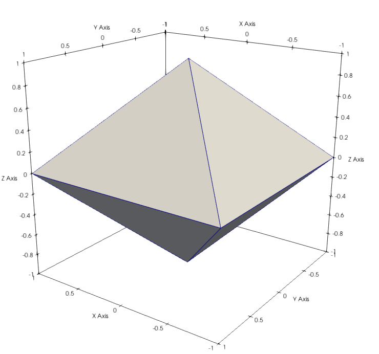
If you see that the 4 first nodes form a square in the \((X,Y)\) plane, and that two other nodes are symetrically located on top and bottom of the center of this square. They are the vertexes of a regular octahedron, which we will verify later by visualizing the mesh.
To get those arrays, the most convenient solution is to use the get_mesh_nodes and get_mesh_nodesID methods:
[9]:
mesh_nodes = data.get_mesh_nodes('mesh')
mesh_nodes_id = data.get_mesh_nodesID('mesh')

for i in range(len(mesh_nodes_id)):
    print(f'Mesh node number {mesh_nodes_id[i]} coordinates: {mesh_nodes[i,:]}')
Mesh node number 0 coordinates: [-1. -1.  0.]
Mesh node number 1 coordinates: [-1.  1.  0.]
Mesh node number 2 coordinates: [1. 1. 0.]
Mesh node number 3 coordinates: [ 1. -1.  0.]
Mesh node number 4 coordinates: [0. 0. 1.]
Mesh node number 5 coordinates: [ 0.  0. -1.]
Node Sets/Tags
You can also see that the Geometry contains a String Array labelled Nodes_tag_list, with item_name NodeTagsList. This group has the following content:
[10]:
data.print_node_info('mesh_NodeTagsList')
 NODE: /test_mesh/Geometry/Node_tags_list
====================
 -- Parent Group : Geometry
 -- Node name : Node_tags_list
 -- Node_tags_list attributes :
         * node_type : string array

 -- content : /test_mesh/Geometry/Node_tags_list (EArray(2,)) ''
 -- Compression options for node `mesh_NodeTagsList`:
        complevel=0, shuffle=False, bitshuffle=False, fletcher32=False, least_significant_digit=None
 --- Chunkshape: (257,)
 -- Node memory size :    63.999 Kb
----------------
You see that this node is a String array, containing 2 elements. They are the names of the NODE SETS, or also NODE TAGS (notation used in SampleData’s code), defined on this mesh, and stored on the dataset. You can access them easily (see String Array section in tutorial 2):
[11]:
for tag in data['mesh_NodeTagsList']:
    print(tag.decode('utf-8'))
Z0_plane
out_of_plane
An easier way to get this information is to use the get_mesh_node_tags method:
[12]:
data.get_mesh_node_tags_names('test_mesh')
[12]:
['Z0_plane', 'out_of_plane']
The two node tags are names Z0_plane, and out_of_plane. From the value of the node coordinates printed a few cells above, we can expect that the Node Set Z0_plane contains the 4 first nodes, and that out_of_plane set the two last nodes.
To see their content, you can use the dedicated methods get_mesh_node_tag and get_mesh_node_tag_coordinates:
[13]:
# Get the node IDs for the Node sets defined on the mesh
Z0_plane = data.get_mesh_node_tag(meshname='test_mesh',node_tag='Z0_plane')
out_of_plane = data.get_mesh_node_tag(meshname='test_mesh',node_tag='out_of_plane')

# Get the node coordinates for the Node sets defined on the mesh
Z0_plane_xyz = data.get_mesh_node_tag_coordinates(meshname='test_mesh',node_tag='Z0_plane')
out_of_plane_xyz = data.get_mesh_node_tag_coordinates(meshname='test_mesh',node_tag='out_of_plane')

# Print informations
print(f'Node tag "Z0_plane" is composed of nodes {Z0_plane} withi coordinates \n {Z0_plane_xyz}','\n')
print(f'Node tag "out_of_plane" is composed of nodes {out_of_plane} withi coordinates \n {out_of_plane_xyz}')
Node tag "Z0_plane" is composed of nodes [0 1 2 3] withi coordinates
 [[-1. -1.  0.]
 [-1.  1.  0.]
 [ 1.  1.  0.]
 [ 1. -1.  0.]]

Node tag "out_of_plane" is composed of nodes [4 5] withi coordinates
 [[ 0.  0.  1.]
 [ 0.  0. -1.]]
The Node Tags are stored in the Group NodeTags, children of the Group Geometry:
[14]:
data.print_node_info('mesh_NodeTags')
data.print_group_content('mesh_NodeTags')
 GROUP NodeTags
=====================
 -- Parent Group : Geometry
 -- Group attributes :
         * group_type : Group
 -- Childrens : NT_Z0_plane, NT_out_of_plane, field_Z0_plane, field_out_of_plane,
----------------


****** Group mesh_NodeTags CONTENT ******


****** Group mesh_NodeTags CONTENT ******

 NODE: /test_mesh/Geometry/NodeTags/NT_Z0_plane
====================
 -- Parent Group : NodeTags
 -- Node name : NT_Z0_plane
 -- NT_Z0_plane attributes :
         * empty : False
         * node_type : data_array

 -- content : /test_mesh/Geometry/NodeTags/NT_Z0_plane (CArray(4,)) 'NT_Z0_plane'
 -- Compression options for node `/test_mesh/Geometry/NodeTags/NT_Z0_plane`:
        complevel=0, shuffle=False, bitshuffle=False, fletcher32=False, least_significant_digit=None
 --- Chunkshape: (8192,)
 -- Node memory size :    64.000 Kb
----------------

 NODE: /test_mesh/Geometry/NodeTags/NT_out_of_plane
====================
 -- Parent Group : NodeTags
 -- Node name : NT_out_of_plane
 -- NT_out_of_plane attributes :
         * empty : False
         * node_type : data_array

 -- content : /test_mesh/Geometry/NodeTags/NT_out_of_plane (CArray(2,)) 'NT_out_of_plane'
 -- Compression options for node `/test_mesh/Geometry/NodeTags/NT_out_of_plane`:
        complevel=0, shuffle=False, bitshuffle=False, fletcher32=False, least_significant_digit=None
 --- Chunkshape: (8192,)
 -- Node memory size :    64.000 Kb
----------------

 NODE: /test_mesh/Geometry/NodeTags/field_Z0_plane
====================
 -- Parent Group : NodeTags
 -- Node name : field_Z0_plane
 -- field_Z0_plane attributes :
         * empty : False
         * field_dimensionality : Scalar
         * field_type : Nodal_field
         * node_type : field_array
         * padding : None
         * parent_grid_path : /test_mesh
         * xdmf_fieldname : field_Z0_plane
         * xdmf_gridname : test_mesh

 -- content : /test_mesh/Geometry/NodeTags/field_Z0_plane (CArray(6, 1), shuffle, zlib(1)) 'mesh_field_Z0_plane'
 -- Compression options for node `/test_mesh/Geometry/NodeTags/field_Z0_plane`:
        complevel=1, complib='zlib', shuffle=True, bitshuffle=False, fletcher32=False, least_significant_digit=None
 --- Chunkshape: (65536, 1)
 -- Node memory size :   310.000 bytes
----------------

 NODE: /test_mesh/Geometry/NodeTags/field_out_of_plane
====================
 -- Parent Group : NodeTags
 -- Node name : field_out_of_plane
 -- field_out_of_plane attributes :
         * empty : False
         * field_dimensionality : Scalar
         * field_type : Nodal_field
         * node_type : field_array
         * padding : None
         * parent_grid_path : /test_mesh
         * xdmf_fieldname : field_out_of_plane
         * xdmf_gridname : test_mesh

 -- content : /test_mesh/Geometry/NodeTags/field_out_of_plane (CArray(6, 1), shuffle, zlib(1)) 'mesh_field_out_of_plane'
 -- Compression options for node `/test_mesh/Geometry/NodeTags/field_out_of_plane`:
        complevel=1, complib='zlib', shuffle=True, bitshuffle=False, fletcher32=False, least_significant_digit=None
 --- Chunkshape: (65536, 1)
 -- Node memory size :   312.000 bytes
----------------
You can observe that the the group contains four data items, two for each node set in our mesh group, as their name indicates.
Two of those data items have a name that starts with ``NT_``, which stand for NodeTag. They contain the data items associated to the node tags, that can be retrieved with the get_mesh_node_tag method (see above).
The two other data item have a name that starts with ``_field``. They are Field Arrays data items. These fields are nodal value fields (see below the section dedicated to Mesh Fields), and have a value of 1 on the node set, and 0 out of the node set.
We have now covered all the elements of the Mesh Group data model related to mesh nodes.
Mesh Elements
Mesh Elements define the geometry of the geometrical domain represented by the grid. They are polylines, polygons or polyhedra whose vertices are mesh Nodes. They are defined by a connectivity array indicating for each element the IDs of the nodes defining the element..
Let us print again the Mesh Group information to find out which data items relate to mesh elements:
[15]:
data.print_node_info('mesh')
 GROUP test_mesh
=====================
 -- Parent Group : /
 -- Group attributes :
         * Elements_offset : [0]
         * Number_of_boundary_elements : [0]
         * Number_of_bulk_elements : [8]
         * Number_of_elements : [8]
         * Topology : Uniform
         * Xdmf_elements_code : ['Triangle']
         * description :
         * element_type : ['tri3']
         * elements_path : /test_mesh/Geometry/Elements
         * empty : False
         * group_type : 3DMesh
         * nodesID_path : /test_mesh/Geometry/Nodes_ID
         * nodes_path : /test_mesh/Geometry/Nodes
         * number_of_nodes : 6
         * xdmf_gridname : test_mesh
 -- Childrens : Geometry, Field_index, Test_field1, Test_field2, Test_field3, Test_field4,
----------------
As shown by this print, many Mesh Group attributes are related to Mesh Elements.
The elements_path attribute indicates the path of the Data Array item containing the elements connectivity array.
The Topology attribute can have two values, Uniform (mesh composed of only one type of elements) or Mixed (mesh composed of several types of elements). Here the mesh is uniform. You will see an example of Mixed topology in the next section of this tutorial. All items of the Mesh Group data Model related to mesh elements will be reviewed again for the Mixed topology case.
Element types
You can see 6 attributes that store list values. All those have one value for each type of element that composes the mesh. Here, as the mesh has a Uniform topology, they have only one value. Two of those attributes provide information on the type of elements:
``elements_type``: a list of the types of elements that is used in the mesh. These type names consist of a geometrical prefix indicating the geometrical nature of the element, followed by a number indicating the number of nodes in the element. Elements types are stored by decreasding dimensionality, in the case of a Mixed topology: the first elements of the lists are the elements types with the higher dimensionality in the mesh (bulk element types), and then element types with a lower dimensionality (boundary element types) are stored. The different type of elements supported, and their dimensionality, are:
Element type
Description
point1A simple point
bar2/bar3A linear/quadratic line segment element (1D)
tri3andtri6A linear/quadratic triangle element (2D)
quad4andquad8A linear/quadratic quadrilateral element (2D)
tet4andtet10A linear/quadratic tetrahedron element (3D)
pyr5andpyr13A linear/quadratic pyramid (square basis) element (3D)
wed6andwed15A linear/quadratic wedge element (3D)
hex8andhex20A linear/quadratic hexaedron element (3D)
``Xdmf_elements_code``: same as
elements_typebut with the element type names of the XDMF data model, that can be found here (used for synchronization with XDMF file)
Note
You will find the geometric definition of these nodes into the BasicTools/Containers/ElementNames.py file of the BasicTools package. They are not presented here for the sake of brevity.
Elements count
Other attributes are used to keep track of the number of elements: Number_of_elements, Number_of_bulk_elements Number_of_boundary_elements. They contain integer values indicating respectively how many elements, bulk elements (i.e. that have the same dimensionality of the mesh, 3D elements for 3D mesh for instance) or boundary elements (elements with a lower dimensionality than the mesh, 2D elements for a 3D mesh for instance) compose the mesh.
These three attributes contain lists, that have a value for each element type of the list, and their order correspond to the element types stored in the elements_type attribute list.
The Elements_offset attribute also is a list with one element per element in elements_type. It contains the position of the first element of each type of element in the complete set of mesh elements. It is used by the class for consistency when interacting with BasicTools Elements objects. It is not relevant for SampleData users.
Using all this information, we can determine that our mesh contains 8 elements, that are linear triangle elements (tri3 elements). They are the 8 faces of our octahedron. A quicker way to retrieve this is to use the get_mesh_elem_types_and_number method, that returns a dictionary whose keys are the element type in the mesh, and values are the number of element for each type:
[16]:
data.get_mesh_elem_types_and_number('mesh')
[16]:
{'tri3': 8}
Elements connectivity array
Like for the Mesh Nodes, all the data describing the Mesh elements is also gathered in the Mesh Geometry Group. Let us print again the content of this group:
[17]:
data.print_group_content('mesh_Geometry', short=True)
data.print_index(local_root='mesh_Geometry')
       --NODE Elem_tag_type_list: /test_mesh/Geometry/Elem_tag_type_list (string array) (   63.999 Kb)
       --NODE Elem_tags_list: /test_mesh/Geometry/Elem_tags_list (string array) (   63.999 Kb)
       --NODE Elements: /test_mesh/Geometry/Elements (data_array) (   64.000 Kb)
      |--GROUP ElementsTags: /test_mesh/Geometry/ElementsTags (Group)
      |--GROUP NodeTags: /test_mesh/Geometry/NodeTags (Group)
       --NODE Node_tags_list: /test_mesh/Geometry/Node_tags_list (string array) (   63.999 Kb)
       --NODE Nodes: /test_mesh/Geometry/Nodes (data_array) (   63.984 Kb)
       --NODE Nodes_ID: /test_mesh/Geometry/Nodes_ID (data_array) (   64.000 Kb)

Dataset Content Index :
------------------------:
index printed with max depth `3` and under local root `mesh_Geometry`

         Name : mesh_ElTagsList                           H5_Path : /test_mesh/Geometry/Elem_tags_list
         Name : mesh_ElTagsTypeList                       H5_Path : /test_mesh/Geometry/Elem_tag_type_list
         Name : mesh_ElemTags                             H5_Path : /test_mesh/Geometry/ElementsTags
         Name : mesh_Elements                             H5_Path : /test_mesh/Geometry/Elements
         Name : mesh_NodeTags                             H5_Path : /test_mesh/Geometry/NodeTags
         Name : mesh_NodeTagsList                         H5_Path : /test_mesh/Geometry/Node_tags_list
         Name : mesh_Nodes                                H5_Path : /test_mesh/Geometry/Nodes
         Name : mesh_Nodes_ID                             H5_Path : /test_mesh/Geometry/Nodes_ID
Like the nodes coordinate array, the element connectivity array is a Data Array node stored into the Mesh Geometry Group. Its item name is Elements. Let us print the content of this array:
[18]:
print(f'The shape of the mesh Elements connectivity array is {data["mesh_Elements"].shape}','\n')
print(f'Its content is {data["mesh_Elements"]}')
The shape of the mesh Elements connectivity array is (24,)

Its content is [0 1 4 0 1 5 1 2 4 1 2 5 2 3 4 2 3 5 3 0 4 3 0 5]
This array contains for each element the IDs of the Nodes that compose the element : 24 nodes IDS, three for each triangle. We can see that the first element of the mesh is composed of the Nodes 0, 1 and 4.
The connectivity array is used as grid Topology array in the XDMF file of the dataset. Hence, it must comply with the XDMF format. For this reason, it is always stored as a 1D array. This format is detailed on the dedicated XDMF data format webpage, `here <https://www.xdmf.org/index.php/XDMF_Model_and_Format#Topology>`__.
In the case of a Uniform topology, the connectivities of the elements are stored consecutively. As the number of nodes of each element is identical, the interpretation of the array is possible. For the Mixed topology case (see example later in this tutorial), the connectivity of each element must be preceded by a number that identifies the element type. This number is the XMDF code for the element type.
The SampleData class offers more convenient ways to get the elements connectivity array. The first is the get_mesh_xdmf_connectivity method, that return the Elements Data array:
[19]:
print(f'The mesh elements connectivity array is {data.get_mesh_xdmf_connectivity("mesh")}')
The mesh elements connectivity array is [0 1 4 0 1 5 1 2 4 1 2 5 2 3 4 2 3 5 3 0 4 3 0 5]
The second is the get_mesh_elements method. With the meshname and one if its element types as arguments, it allows to get the connectivity of a type of elements with a classical 2D array format:
[20]:
data.get_mesh_elements(meshname='mesh', get_eltype_connectivity='tri3')
[20]:
array([[0, 1, 4],
       [0, 1, 5],
       [1, 2, 4],
       [1, 2, 5],
       [2, 3, 4],
       [2, 3, 5],
       [3, 0, 4],
       [3, 0, 5]])
Elements Sets/Tags
Like Node Tags, Mesh Group can store Element Tags (= element sets) in the Mesh Geometry Group), that are stored in the ElementsTags Group, and listed in the ElTagsList String array. A second string array is associated to element tags: the ElTagsTypeList that contains the type of element constituting each tag (element tags can only be composed of a single type of elements). Like for node tags, they are explicit methods that allow to retrieve information on element tags:
[21]:
data.get_mesh_elem_tags_names('mesh')
[21]:
{'2D': 'tri3', 'Top': 'tri3', 'Bottom': 'tri3'}
Our Mesh Group contains 3 element tags, all containing tri3 elements. The elements IDs and the specific connectivity of an element tag can easily be accessed using their name and the Mesh Group name:
[22]:
el_tag = data.get_mesh_elem_tag(meshname='mesh', element_tag='2D')
el_tag_connect = data.get_mesh_elem_tag_connectivity(meshname='mesh', element_tag='Bottom')
# el_tag_connect = data.get_mesh_elem_tags_connectivity(meshname='mesh', element_tag='2D')

print(f'The element tag `2D` contains the elements: {el_tag}.')
print(f'The connectivity of the `Bottom` element tag is: \n {el_tag_connect}')
The element tag `2D` contains the elements: [0 1 2 3 4 5 6 7].
The connectivity of the `Bottom` element tag is:
 [[0 1 5]
 [1 2 5]
 [2 3 5]
 [3 0 5]]
You can observe that the get_mesh_elem_tag_connectivity reshapes the connectivity array to a more usual 2D format, each row of the array corresponding to the connectivity of 1 element.
Like for Node Tags, the arrays containing the Element Tags data are stored in a specific group ElementsTags, subgroup of the Mesh Geometry Group. They contain the ID numbers of the elements constituting the Element Tag, and are named following the pattern : ET_+tag name (ET standing for element tag).
Like for Nodes, Mesh Groups can also store Mesh fields for Element Tags to allow to visualize them. These fields have one boolean value per mesh element, which is equal to 1 on elements that are part of the Element Tag. The associated data arrays are also stored in the ElementsTags Group, and are named following the pattern : field_+tag name.
Let us look at the content of this Group:
[23]:
data.print_group_content('mesh_ElemTags')
****** Group mesh_ElemTags CONTENT ******


****** Group mesh_ElemTags CONTENT ******

 NODE: /test_mesh/Geometry/ElementsTags/ET_2D
====================
 -- Parent Group : ElementsTags
 -- Node name : ET_2D
 -- ET_2D attributes :
         * empty : False
         * node_type : data_array

 -- content : /test_mesh/Geometry/ElementsTags/ET_2D (CArray(8,)) 'ET_2D'
 -- Compression options for node `/test_mesh/Geometry/ElementsTags/ET_2D`:
        complevel=0, shuffle=False, bitshuffle=False, fletcher32=False, least_significant_digit=None
 --- Chunkshape: (8192,)
 -- Node memory size :    64.000 Kb
----------------

 NODE: /test_mesh/Geometry/ElementsTags/ET_Bottom
====================
 -- Parent Group : ElementsTags
 -- Node name : ET_Bottom
 -- ET_Bottom attributes :
         * empty : False
         * node_type : data_array

 -- content : /test_mesh/Geometry/ElementsTags/ET_Bottom (CArray(4,)) 'ET_Bottom'
 -- Compression options for node `/test_mesh/Geometry/ElementsTags/ET_Bottom`:
        complevel=0, shuffle=False, bitshuffle=False, fletcher32=False, least_significant_digit=None
 --- Chunkshape: (8192,)
 -- Node memory size :    64.000 Kb
----------------

 NODE: /test_mesh/Geometry/ElementsTags/ET_Top
====================
 -- Parent Group : ElementsTags
 -- Node name : ET_Top
 -- ET_Top attributes :
         * empty : False
         * node_type : data_array

 -- content : /test_mesh/Geometry/ElementsTags/ET_Top (CArray(4,)) 'ET_Top'
 -- Compression options for node `/test_mesh/Geometry/ElementsTags/ET_Top`:
        complevel=0, shuffle=False, bitshuffle=False, fletcher32=False, least_significant_digit=None
 --- Chunkshape: (8192,)
 -- Node memory size :    64.000 Kb
----------------

 NODE: /test_mesh/Geometry/ElementsTags/field_2D
====================
 -- Parent Group : ElementsTags
 -- Node name : field_2D
 -- field_2D attributes :
         * empty : False
         * field_dimensionality : Scalar
         * field_type : Element_field
         * node_type : field_array
         * padding : bulk
         * parent_grid_path : /test_mesh
         * xdmf_fieldname : field_2D
         * xdmf_gridname : test_mesh

 -- content : /test_mesh/Geometry/ElementsTags/field_2D (CArray(8, 1), shuffle, zlib(1)) 'mesh_field_2D'
 -- Compression options for node `/test_mesh/Geometry/ElementsTags/field_2D`:
        complevel=1, complib='zlib', shuffle=True, bitshuffle=False, fletcher32=False, least_significant_digit=None
 --- Chunkshape: (8192, 1)
 -- Node memory size :   325.000 bytes
----------------

 NODE: /test_mesh/Geometry/ElementsTags/field_Bottom
====================
 -- Parent Group : ElementsTags
 -- Node name : field_Bottom
 -- field_Bottom attributes :
         * empty : False
         * field_dimensionality : Scalar
         * field_type : Element_field
         * node_type : field_array
         * padding : bulk
         * parent_grid_path : /test_mesh
         * xdmf_fieldname : field_Bottom
         * xdmf_gridname : test_mesh

 -- content : /test_mesh/Geometry/ElementsTags/field_Bottom (CArray(8, 1), shuffle, zlib(1)) 'mesh_field_Bottom'
 -- Compression options for node `/test_mesh/Geometry/ElementsTags/field_Bottom`:
        complevel=1, complib='zlib', shuffle=True, bitshuffle=False, fletcher32=False, least_significant_digit=None
 --- Chunkshape: (8192, 1)
 -- Node memory size :   328.000 bytes
----------------

 NODE: /test_mesh/Geometry/ElementsTags/field_Top
====================
 -- Parent Group : ElementsTags
 -- Node name : field_Top
 -- field_Top attributes :
         * empty : False
         * field_dimensionality : Scalar
         * field_type : Element_field
         * node_type : field_array
         * padding : bulk
         * parent_grid_path : /test_mesh
         * xdmf_fieldname : field_Top
         * xdmf_gridname : test_mesh

 -- content : /test_mesh/Geometry/ElementsTags/field_Top (CArray(8, 1), shuffle, zlib(1)) 'mesh_field_Top'
 -- Compression options for node `/test_mesh/Geometry/ElementsTags/field_Top`:
        complevel=1, complib='zlib', shuffle=True, bitshuffle=False, fletcher32=False, least_significant_digit=None
 --- Chunkshape: (8192, 1)
 -- Node memory size :   327.000 bytes
----------------
We see that our 3 element tags have a field associated in the Mesh Group.
Mesh fields
Like Image Groups, Mesh Groups can store fields. The list of the names of fields defined on the mesh group is stored in the Field_Index string array, like for Image Groups ( see previous tutorial). It can be accessed easily using the get_grid_field_list method:
[24]:
data.get_grid_field_list('mesh')
[24]:
['mesh_field_Z0_plane',
 'mesh_field_out_of_plane',
 'mesh_field_2D',
 'mesh_field_Top',
 'mesh_field_Bottom',
 'mesh_Test_field1',
 'mesh_Test_field2',
 'mesh_Test_field3',
 'mesh_Test_field4']
We see in this list the various Node/Element tag fields, but also additional fields called mesh_test_fieldX. A specific section is dedicated to Mesh fields in this tutorial, so no additional detail on them will be provided here.
Mesh XDMF grids
We have now seen all the data contained in a Mesh Group in the HDF5 dataset of a SampleData object. To conclude this section on the Mesh Group data model, we will observe how this group is stored in the XDMF dataset:
[25]:
data.print_xdmf()
<!DOCTYPE Xdmf SYSTEM "Xdmf.dtd">
<Xdmf xmlns:xi="http://www.w3.org/2003/XInclude" Version="2.2">
  <Domain>
    <Grid Name="test_mesh" GridType="Uniform">
      <Geometry Type="XYZ">
        <DataItem Format="HDF" Dimensions="6  3" NumberType="Float" Precision="64">test_sampledata_ref.h5:/test_mesh/Geometry/Nodes</DataItem>
      </Geometry>
      <Topology TopologyType="Triangle" NumberOfElements="8">
        <DataItem Format="HDF" Dimensions="24 " NumberType="Int" Precision="64">test_sampledata_ref.h5:/test_mesh/Geometry/Elements</DataItem>
      </Topology>
      <Attribute Name="field_Z0_plane" AttributeType="Scalar" Center="Node">
        <DataItem Format="HDF" Dimensions="6  1" NumberType="Int" Precision="8">test_sampledata_ref.h5:/test_mesh/Geometry/NodeTags/field_Z0_plane</DataItem>
      </Attribute>
      <Attribute Name="field_out_of_plane" AttributeType="Scalar" Center="Node">
        <DataItem Format="HDF" Dimensions="6  1" NumberType="Int" Precision="8">test_sampledata_ref.h5:/test_mesh/Geometry/NodeTags/field_out_of_plane</DataItem>
      </Attribute>
      <Attribute Name="field_2D" AttributeType="Scalar" Center="Cell">
        <DataItem Format="HDF" Dimensions="8  1" NumberType="Float" Precision="64">test_sampledata_ref.h5:/test_mesh/Geometry/ElementsTags/field_2D</DataItem>
      </Attribute>
      <Attribute Name="field_Top" AttributeType="Scalar" Center="Cell">
        <DataItem Format="HDF" Dimensions="8  1" NumberType="Float" Precision="64">test_sampledata_ref.h5:/test_mesh/Geometry/ElementsTags/field_Top</DataItem>
      </Attribute>
      <Attribute Name="field_Bottom" AttributeType="Scalar" Center="Cell">
        <DataItem Format="HDF" Dimensions="8  1" NumberType="Float" Precision="64">test_sampledata_ref.h5:/test_mesh/Geometry/ElementsTags/field_Bottom</DataItem>
      </Attribute>
      <Attribute Name="Test_field1" AttributeType="Scalar" Center="Node">
        <DataItem Format="HDF" Dimensions="6  1" NumberType="Float" Precision="64">test_sampledata_ref.h5:/test_mesh/Test_field1</DataItem>
      </Attribute>
      <Attribute Name="Test_field2" AttributeType="Scalar" Center="Node">
        <DataItem Format="HDF" Dimensions="6  1" NumberType="Float" Precision="64">test_sampledata_ref.h5:/test_mesh/Test_field2</DataItem>
      </Attribute>
      <Attribute Name="Test_field3" AttributeType="Scalar" Center="Cell">
        <DataItem Format="HDF" Dimensions="8  1" NumberType="Float" Precision="64">test_sampledata_ref.h5:/test_mesh/Test_field3</DataItem>
      </Attribute>
      <Attribute Name="Test_field4" AttributeType="Scalar" Center="Cell">
        <DataItem Format="HDF" Dimensions="8  1" NumberType="Float" Precision="64">test_sampledata_ref.h5:/test_mesh/Test_field4</DataItem>
      </Attribute>
    </Grid>
    <Grid Name="test_image" GridType="Uniform">
      <Topology TopologyType="3DCoRectMesh" Dimensions="10 10 10"/>
      <Geometry Type="ORIGIN_DXDYDZ">
        <DataItem Format="XML" Dimensions="3">-1. -1. -1.</DataItem>
        <DataItem Format="XML" Dimensions="3">0.2 0.2 0.2</DataItem>
      </Geometry>
      <Attribute Name="test_image_field" AttributeType="Scalar" Center="Node">
        <DataItem Format="HDF" Dimensions="10  10  10" NumberType="Int" Precision="16">test_sampledata_ref.h5:/test_image/test_image_field</DataItem>
      </Attribute>
    </Grid>
  </Domain>
</Xdmf>
You can see that the test_mesh is stored as a Grid Node. This node contains a Geometry node, defined by a data array, which is the Node coordinate data array stored in the HDF5 dataset. It also contains a Topology Group, defined by the Elements connectivity data array stored in the HDF5 dataset. Finally, it contains one Attribute node for each field listed in the Field Index string array of the HDF5 dataset, defined by the associated data array in the HDF5 dataset.
As already explained in the tutorial 1 (sec. V), the XDMF file allows to directly visualize the data described in it with the Paraview software. Before closing our reference dataset, Let us try to visualize the Mesh Group that we have studied, with the pause_for_visualization method and the Paraview software.
You have to choose the XdmfReader to open the file, so that Paraview may properly read the data. In the Property panel, tick only the test_mesh block to only plot the content of the Mesh Group, and then click on the Apply button.
[26]:
# Use the second code line if you want to specify the path of the paraview executable you want to use
# otherwise use the first line
#data.pause_for_visualization(Paraview=True)
#data.pause_for_visualization(Paraview=True, Paraview_path='path to paraview executable')
You should be able to produce visualization of the mesh geometry:
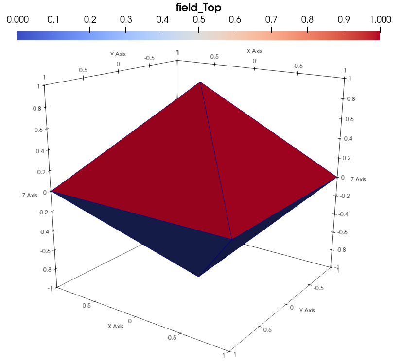
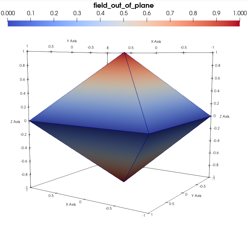
or the mesh fields:
Before moving to the next section on the creation of Mesh Groups, let us close our reference dataset:
[27]:
del data
III - Creating Mesh Groups
Like for Image Groups (see tutorial 4 section III), Mesh Groups are created in SampleData instances through Basictools mesh objects. Creating meshes is a complex geometrical and mathematical task, that require specific tools (meshers like gmsh for instance). The SampleData code has not been designed to create meshes, but rather to manipulate them. In relevant application of the class, mesh data stored into SampleData datasets come from external tools. The main tasks are then to load and manipulate the data. This tutorial will mainly focus on those aspect, rather than mesh creation.
Hence, in this section, we will only review some quick ways to create mesh objects, from simple mesh data, mesh files or other Python packages; and how to add them to a SampleData dataset.
Creating mesh objects with BasicTools
The BasicTools package implements a few methods that allow to create meshes with simple topologies. We will rely on them to recreate the mesh that we studied before, and introduce you to mesh objects.
BasicTools mesh creation tools
The mesh creation tools of the BasicTools package can be imported with the following code line:
[28]:
import BasicTools.Containers.UnstructuredMeshCreationTools as UMCT
This module contains functions that allow, from a set of points and a connectivity matrix, to create uniform meshes of one type of element. Learning in details how to use them is beyond the scope of this tutorial. Likewise, how to add data such as tags or fields to a mesh object will not be detailed in this tutorial. The reader is refered to BasicTools code to learn more on those methods/objects.
These method include:
CreateUniformMeshOfBarsCreateMeshOfTrianglesCreateMeshOfCreateSquareCreateCubeCreateMeshFromConstantRectilinearMesh
The UnstructuredMeshCreationTools contains test methods for each of these methods that can be read to understand how to use them.
To recreate the octahedron mesh of the reference dataset studied in section II, we will use the CreateMeshOfTriangles method. For that, we will need to create two arrays, one for the node coordinates, one for the elements connectivity, and simply pass them to the BasicTools method:
[29]:
import numpy as np
# Mesh node coordinates array
mesh_nodes = np.array([[-1.,-1., 0.],
                       [-1., 1., 0.],
                       [ 1., 1., 0.],
                       [ 1.,-1., 0.],
                       [ 0., 0., 1.],
                       [ 0., 0.,-1.]])
# Mesh connectivity array
mesh_elements = np.array([[0, 1, 4],
                          [0, 1, 5],
                          [1, 2, 4],
                          [1, 2, 5],
                          [2, 3, 4],
                          [2, 3, 5],
                          [3, 0, 4],
                          [3, 0, 5]])
mesh = UMCT.CreateMeshOfTriangles(mesh_nodes, mesh_elements)
Mesh objects
The method return a BasicTools unstructured mesh object, a class dedicated to the manipulation of finite element meshes data. Printing this object provides information on the content of the mesh:
[30]:
print(mesh)
UnstructuredMesh
  Number Of Nodes    : 6
    Tags :
  Number Of Elements : 8
    ElementsContainer,   Type : (tri3,8),   Tags : (2D:8)
We will now complete this mesh object with additional data, by defining fields and node/element tags:
[31]:
# Here we recreate the Node tags of the reference dataset `test_mesh`
mesh.nodesTags.CreateTag('Z0_plane', False).SetIds([0,1,2,3])
mesh.nodesTags.CreateTag('out_of_plane', False).SetIds([4,5])

# Here we recreate the Element tags of the reference dataset `test_mesh`
mesh.GetElementsOfType('tri3').GetTag('Top').SetIds([0,2,4,6])
mesh.GetElementsOfType('tri3').GetTag('Bottom').SetIds([1,3,5,7])

# Here we add mesh node fields
mesh.nodeFields['Test_field1'] = np.array([0., 0., 0., 0., 1., 0.])
mesh.nodeFields['Test_field2'] = np.array([0., 0., 0., 0., 0., 1.])
# Here we add mesh element fields
mesh.elemFields['Test_field3'] = np.array([0., 1., 2., 3., 4., 5., 6., 7.])
mesh.elemFields['Test_field4'] = np.array([1., 1., -1., -1., 1., 1., -1., -1.])
[32]:
print(mesh)
UnstructuredMesh
  Number Of Nodes    : 6
    Tags : (Z0_plane:4) (out_of_plane:2)
  Number Of Elements : 8
    ElementsContainer,   Type : (tri3,8),   Tags : (2D:8) (Top:4) (Bottom:4)
  nodeFields         : ['Test_field1', 'Test_field2']
  elemFields         : ['Test_field3', 'Test_field4']
Creating a Mesh Group from a Meshobject
Our mesh object now contain all the data that is stored into the test_mesh Group of the reference dataset. We can now create a new Sampledata instance to see how we can create a MeshGroup from this mesh object:
[33]:
data = SD(filename='test_mesh_dataset', overwrite_hdf5=True, autodelete=True)
To add a Mesh Group into this dataset, use the add_mesh method. Its use is very straightforward, you just have to provide the name, indexname, location of the Mesh Group you want to create, and the mesh object from which the data must be loaded. Like all the data item creation methods, it also has a replace argument (see tutorial 3).
This methods has one specific argument, bin_fields_from_sets, that allow you to control if you want to simply store the Node/Element Tags as data arrays (in this case set it to False), or if you want to also store visualization fields for each Node/Element Tag in the mesh object.
Let us create our mesh group, with visualization fields:
[34]:
data.add_mesh(mesh_object=mesh, meshname='test_mesh', indexname='mesh', location='/', bin_fields_from_sets=True)
[34]:
<BasicTools.Containers.UnstructuredMesh.UnstructuredMesh at 0x7fc308414b90>
[35]:
print(data)
Dataset Content Index :
------------------------:
index printed with max depth `3` and under local root `/`

         Name : mesh                                      H5_Path : /test_mesh
         Name : mesh_Geometry                             H5_Path : /test_mesh/Geometry
         Name : mesh_Nodes                                H5_Path : /test_mesh/Geometry/Nodes
         Name : mesh_Nodes_ID                             H5_Path : /test_mesh/Geometry/Nodes_ID
         Name : mesh_Elements                             H5_Path : /test_mesh/Geometry/Elements
         Name : mesh_NodeTags                             H5_Path : /test_mesh/Geometry/NodeTags
         Name : mesh_Field_index                          H5_Path : /test_mesh/Field_index
         Name : mesh_NodeTagsList                         H5_Path : /test_mesh/Geometry/Node_tags_list
         Name : mesh_ElemTags                             H5_Path : /test_mesh/Geometry/ElementsTags
         Name : mesh_ElTagsList                           H5_Path : /test_mesh/Geometry/Elem_tags_list
         Name : mesh_ElTagsTypeList                       H5_Path : /test_mesh/Geometry/Elem_tag_type_list
         Name : mesh_Test_field1                          H5_Path : /test_mesh/Test_field1
         Name : mesh_Test_field2                          H5_Path : /test_mesh/Test_field2
         Name : mesh_Test_field3                          H5_Path : /test_mesh/Test_field3
         Name : mesh_Test_field4                          H5_Path : /test_mesh/Test_field4

Printing dataset content with max depth 3
  |--GROUP test_mesh: /test_mesh (3DMesh)
     --NODE Field_index: /test_mesh/Field_index (string_array - empty) (   63.999 Kb)
    |--GROUP Geometry: /test_mesh/Geometry (Group)
       --NODE Elem_tag_type_list: /test_mesh/Geometry/Elem_tag_type_list (string_array) (   63.999 Kb)
       --NODE Elem_tags_list: /test_mesh/Geometry/Elem_tags_list (string_array) (   63.999 Kb)
       --NODE Elements: /test_mesh/Geometry/Elements (data_array) (   64.000 Kb)
      |--GROUP ElementsTags: /test_mesh/Geometry/ElementsTags (Group)
      |--GROUP NodeTags: /test_mesh/Geometry/NodeTags (Group)
       --NODE Node_tags_list: /test_mesh/Geometry/Node_tags_list (string_array) (   63.999 Kb)
       --NODE Nodes: /test_mesh/Geometry/Nodes (data_array) (   63.984 Kb)
       --NODE Nodes_ID: /test_mesh/Geometry/Nodes_ID (data_array) (   64.000 Kb)

     --NODE Test_field1: /test_mesh/Test_field1 (field_array) (   64.000 Kb)
     --NODE Test_field2: /test_mesh/Test_field2 (field_array) (   64.000 Kb)
     --NODE Test_field3: /test_mesh/Test_field3 (field_array) (   64.000 Kb)
     --NODE Test_field4: /test_mesh/Test_field4 (field_array) (   64.000 Kb)
That is it ! The Mesh Group has been created and all data has been stored into the SampleData dataset. Let us try to retrieve some information to check the loaded data:
[36]:
data.print_node_info('mesh_Geometry')
print('Mesh elements: ',data.get_mesh_elem_types_and_number('mesh'))
print('Mesh node tags: ', data.get_mesh_node_tags_names('mesh'))
print('Mesh element tags:',data.get_mesh_elem_tags_names('mesh'))
print('Element Tag "Bottom" connectivity: \n',data.get_mesh_elem_tag_connectivity('mesh', 'Bottom'))
 GROUP Geometry
=====================
 -- Parent Group : test_mesh
 -- Group attributes :
         * group_type : Group
 -- Childrens : Nodes, Nodes_ID, Elements, NodeTags, Node_tags_list, ElementsTags, Elem_tags_list, Elem_tag_type_list,
----------------

Mesh elements:  {'tri3': 8}
Mesh node tags:  ['Z0_plane', 'out_of_plane']
Mesh element tags: {'2D': 'tri3', 'Top': 'tri3', 'Bottom': 'tri3'}
Element Tag "Bottom" connectivity:
 [[0 1 5]
 [1 2 5]
 [2 3 5]
 [3 0 5]]
Creating meshes from files
In practice, creating relevant meshes for mechanical or material science application through BasicTools mesh creation tools is very limited. The most relevant use case consist in loading meshes from mesh files created by finite element or meshing softwares. Through Basictools, the SampleData class allows to directly load Mesh Groups from various mesh file formats, and the opposite: write mesh files in various formats from Mesh Groups.
Load mesh files
We will use a mesh file used for Pymicro unit tests to illustrate the mesh file loading functionality. This file is a .geof file, the mesh file format used by the Zset finite element software.
To load a mesh file from into a SampleData mesh group, use the add_mesh method, but instead of providing a mesh object, use the file argument and provide the mesh file name:
[37]:
meshfile_name = os.path.join(PYMICRO_EXAMPLES_DATA_DIR, 'cube_ref.geof')
print(meshfile_name)

data.add_mesh(file=meshfile_name, meshname='loaded_geof_mesh', indexname='mesh_geof', location='/', bin_fields_from_sets=True)

print(data)
/home/amarano/Codes/pymicro/examples/data/cube_ref.geof
Dataset Content Index :
------------------------:
index printed with max depth `3` and under local root `/`

         Name : mesh                                      H5_Path : /test_mesh
         Name : mesh_Geometry                             H5_Path : /test_mesh/Geometry
         Name : mesh_Nodes                                H5_Path : /test_mesh/Geometry/Nodes
         Name : mesh_Nodes_ID                             H5_Path : /test_mesh/Geometry/Nodes_ID
         Name : mesh_Elements                             H5_Path : /test_mesh/Geometry/Elements
         Name : mesh_NodeTags                             H5_Path : /test_mesh/Geometry/NodeTags
         Name : mesh_Field_index                          H5_Path : /test_mesh/Field_index
         Name : mesh_NodeTagsList                         H5_Path : /test_mesh/Geometry/Node_tags_list
         Name : mesh_ElemTags                             H5_Path : /test_mesh/Geometry/ElementsTags
         Name : mesh_ElTagsList                           H5_Path : /test_mesh/Geometry/Elem_tags_list
         Name : mesh_ElTagsTypeList                       H5_Path : /test_mesh/Geometry/Elem_tag_type_list
         Name : mesh_Test_field1                          H5_Path : /test_mesh/Test_field1
         Name : mesh_Test_field2                          H5_Path : /test_mesh/Test_field2
         Name : mesh_Test_field3                          H5_Path : /test_mesh/Test_field3
         Name : mesh_Test_field4                          H5_Path : /test_mesh/Test_field4
         Name : mesh_geof                                 H5_Path : /loaded_geof_mesh
         Name : mesh_geof_Geometry                        H5_Path : /loaded_geof_mesh/Geometry
         Name : mesh_geof_Nodes                           H5_Path : /loaded_geof_mesh/Geometry/Nodes
         Name : mesh_geof_Nodes_ID                        H5_Path : /loaded_geof_mesh/Geometry/Nodes_ID
         Name : mesh_geof_Elements                        H5_Path : /loaded_geof_mesh/Geometry/Elements
         Name : mesh_geof_NodeTags                        H5_Path : /loaded_geof_mesh/Geometry/NodeTags
         Name : mesh_geof_Field_index                     H5_Path : /loaded_geof_mesh/Field_index
         Name : mesh_geof_NodeTagsList                    H5_Path : /loaded_geof_mesh/Geometry/Node_tags_list
         Name : mesh_geof_ElemTags                        H5_Path : /loaded_geof_mesh/Geometry/ElementsTags
         Name : mesh_geof_ElTagsList                      H5_Path : /loaded_geof_mesh/Geometry/Elem_tags_list
         Name : mesh_geof_ElTagsTypeList                  H5_Path : /loaded_geof_mesh/Geometry/Elem_tag_type_list

Printing dataset content with max depth 3
  |--GROUP loaded_geof_mesh: /loaded_geof_mesh (3DMesh)
     --NODE Field_index: /loaded_geof_mesh/Field_index (string_array - empty) (   63.999 Kb)
    |--GROUP Geometry: /loaded_geof_mesh/Geometry (Group)
       --NODE Elem_tag_type_list: /loaded_geof_mesh/Geometry/Elem_tag_type_list (string_array) (   63.999 Kb)
       --NODE Elem_tags_list: /loaded_geof_mesh/Geometry/Elem_tags_list (string_array) (   63.999 Kb)
       --NODE Elements: /loaded_geof_mesh/Geometry/Elements (data_array) (   64.000 Kb)
      |--GROUP ElementsTags: /loaded_geof_mesh/Geometry/ElementsTags (Group)
      |--GROUP NodeTags: /loaded_geof_mesh/Geometry/NodeTags (Group)
       --NODE Node_tags_list: /loaded_geof_mesh/Geometry/Node_tags_list (string_array) (   63.999 Kb)
       --NODE Nodes: /loaded_geof_mesh/Geometry/Nodes (data_array) (   63.984 Kb)
       --NODE Nodes_ID: /loaded_geof_mesh/Geometry/Nodes_ID (data_array) (   64.000 Kb)


  |--GROUP test_mesh: /test_mesh (3DMesh)
     --NODE Field_index: /test_mesh/Field_index (string_array - empty) (   63.999 Kb)
    |--GROUP Geometry: /test_mesh/Geometry (Group)
       --NODE Elem_tag_type_list: /test_mesh/Geometry/Elem_tag_type_list (string_array) (   63.999 Kb)
       --NODE Elem_tags_list: /test_mesh/Geometry/Elem_tags_list (string_array) (   63.999 Kb)
       --NODE Elements: /test_mesh/Geometry/Elements (data_array) (   64.000 Kb)
      |--GROUP ElementsTags: /test_mesh/Geometry/ElementsTags (Group)
      |--GROUP NodeTags: /test_mesh/Geometry/NodeTags (Group)
       --NODE Node_tags_list: /test_mesh/Geometry/Node_tags_list (string_array) (   63.999 Kb)
       --NODE Nodes: /test_mesh/Geometry/Nodes (data_array) (   63.984 Kb)
       --NODE Nodes_ID: /test_mesh/Geometry/Nodes_ID (data_array) (   64.000 Kb)

     --NODE Test_field1: /test_mesh/Test_field1 (field_array) (   64.000 Kb)
     --NODE Test_field2: /test_mesh/Test_field2 (field_array) (   64.000 Kb)
     --NODE Test_field3: /test_mesh/Test_field3 (field_array) (   64.000 Kb)
     --NODE Test_field4: /test_mesh/Test_field4 (field_array) (   64.000 Kb)
The Mesh Group has been loaded as a Mesh Group in the dataset. Its data can be explored, and visualized, as presented above:
[38]:
data.print_node_info('mesh_geof')
print('Mesh elements: ',data.get_mesh_elem_types_and_number('mesh_geof'))
print('Mesh node tags: ', data.get_mesh_node_tags_names('mesh_geof'))
print('Mesh element tags:',data.get_mesh_elem_tags_names('mesh_geof'))
 GROUP loaded_geof_mesh
=====================
 -- Parent Group : /
 -- Group attributes :
         * Elements_offset : [  0 384]
         * Number_of_boundary_elements : [384]
         * Number_of_bulk_elements : [384]
         * Number_of_elements : [384 384]
         * Topology : Mixed
         * Xdmf_elements_code : [6, 4]
         * description :
         * element_type : ['tet4', 'tri3']
         * elements_path : /loaded_geof_mesh/Geometry/Elements
         * empty : False
         * group_type : 3DMesh
         * nodesID_path : /loaded_geof_mesh/Geometry/Nodes_ID
         * nodes_path : /loaded_geof_mesh/Geometry/Nodes
         * number_of_nodes : 125
         * xdmf_gridname : loaded_geof_mesh
 -- Childrens : Geometry, Field_index,
----------------

Mesh elements:  {'tet4': 384, 'tri3': 384}
Mesh node tags:  ['x0y0z0', 'x1y0z0', 'x0y1z0', 'x1y1z0', 'x0y0z1', 'x1y0z1', 'x0y1z1', 'x1y1z1']
Mesh element tags: {'3D': 'tet4', 'X0': 'tri3', 'Y0': 'tri3', 'Skin': 'tri3', 'X1': 'tri3', 'Y1': 'tri3', 'Z0': 'tri3', 'Z1': 'tri3'}
As you can see, this mesh has a mixed topology, and has bulk (linear tetrahedra tet4) and boundary (linear triangles tri3) elements. This is the mesh of a cube, and it contains element tags to define its faces (X0, X1, Y0 …). As a training exercise, you may try to explore and visualize all the data contained into this mesh group !
This method will in principle work with the following files extensions :
.geof .inp, .asc, .ansys, .geo, .msh, .mesh, .meshb, .sol, .solb, .gcode, .fem, .stl, .xdmf, .pxdmf, .PIPE, .odb, .ut, .utp, .vtu, .dat, .datt
Note: MeshIO Bridge
If you use the meshio package to handle meshes, you can interface it with SampleData thanks to the BasicTools package. For that, you can use the MeshToMeshIO and MeshIOToMesh methods in the BasicTools.Containers.MeshIOBridge module of the Basictools package. These methods allow you to transform a Basictools mesh object into a MeshIO object. Hence, you can load a meshio mesh into a SampleData dataset by transforming it into a Basictools mesh object, and feeding it to
the add_mesh method.
IV - Mesh Field data model
In this new section, we will now focus on the definition of mesh fields data items. They are very similar to image fields data items, presented in the previous tutorial, section IV. They are data arrays enriched with metadata describing how they relate to the mesh they are associated to. Like image fields, these data arrays must follow some shape, ordering and indexing conventions to be added as mesh fields.
SampleData Mesh fields conventions
Possible shapes and field types
In the following, \(N_n\), \(N_e\) and \(N_{ip}\) represent respectively the number of nodes, elements and intergration points of the mesh. Mesh fields can be added from Numpy array that can have the following shapes:
\((N_n, N_c)\) or \((N_n)\) (equivalent to \(N_c=1\)). In this case, the field is a nodal field, whose values are defined at the mesh nodes
\((N_e, N_c)\) or \((N_e)\) (equivalent to \(N_c=1\)). In this case, the field is an element field, whose values are defined on each mesh element (constant per element)
\((N_{ip},N_c)\) or \((N_{ip})\) (equivalent to \(N_c=1\)). In this case, the field is an integration point field, whose values are defined at the mesh integration points. In practice, \(N_{ip}\) can be any multiple of \(N_e\), \(N_{ip} = k*N_e\)
If an array that do not have a compatible shape is added as mesh field, the class will raise an exception.
Field padding
Finite element softwares may output fields only on bulk elements or boundary elements (variable flux, pressure field…) depending on the field nature. If such field must be loaded into a SampleData Mesh Group that has a mixed topology, with bulk and boundary elements, an element or integration point field array outputed by the software will not have a number of values compliant with the convention presented in the subsection above.
The SampleData class handles automatically this particular issue. Element and integration point fields may be added from field data that are defined only on bulk or boundary elements. The class will padd them with zeros values for the element over which they are not defined, to get the proper array size.
In practice, to add element fields / integration point fields, the input array can have the shape \((N_e, N_c)\) or \((N_e)\) / \((N_{ip}, N_c)\) or \((N_{ip})\), with \(N_{ip} = k*N_e\) and \(N_e\) being either the total number of elements in the mesh, the number of bulk elements in the mesh, or the number of boundary elements in the mesh.
Integration points ordering convention and visualization
For each component of the field, integration point field array values are ordered by increasing integration point index first, and then by increasing element index, as follows:
\(Array[:,c] = [A_{ip1/e1}, A_{ip2/e1}, ..., A_{ip1/e2}, ...,A_{ipM/eN} ]\)
where \(A_{ipi/ej}\) denotes the value of the array \(A\) for the integration point \(i\) of the element \(j\), and \(M\) and \(N\) are respectively the number of integration point per element and the number of elements in the mesh.
The XDMF format does not allow to specify integration points values for grids, and hence, these values cannot be directly visualized with Paraview and SampleData dataset yet. However, when adding a an integration point field to a dataset, the user may chose to associate to it a visualization field that is an element field (1 value per element), which is the minimum, maximum or mean of the field value on all element integration points (see next section).
Field dimensionality
The size of the last dimension of the array determines the number of field components \(N_c\), which defines the field dimensionality. If the array is 1D, then \(N_c=1\).
SampleData will interpret the field dimensionality (scalar, vector, or tensor) depending on the grid topology and the array shape. All possibilities are listed hereafter: * \(N_c=1\): scalar field * \(N_c=3\): vector field * \(N_c=6\): symetric tensor field (2nd order tensor) * \(N_c=9\): tensor field (2nd order tensor)
The dimensionality of the field has the following implications: * XDMF: the dimensionality of the field is one of the metadata stored in the XDMF file, for Fields (Attribute nodes) * visualization: as it is stored in the XDMF file, Paraview can correctly interpret the fields according to their dimensionality. Il allows to plot separately each field component, and the field norm (magnitude). It also allows to use the Paraview Glyph filter to plot vector fields with arrows *
indexing: The order of the value in the last dimension for non-scalar fields correspond to a specific order of the field components, according to a specific convention. These conventions will be detailed in the next subsection. * compression: Specific lossy compression options exist for fields. See dedicated tutorial. * interface with external tools: when interfacing SampleData with external softwares, such as numerical simulation tools, it is very practical to have fields with
appropriate dimensionality accounted for (for instance to use a displacement or temperature gradient vector field stored in a SampleData dataset as input for a finite element simulation).
Field components indexing
To detail the convention, we will omit the spatial indexes \(i,j\) or \(k\) and only consider the last dimension of the field: \(F[i,c] = F[c]\). The indexing convention to describe field components order in data arrays are:
For vector fields (3 components), the convention is \([F_0,F_1,F_2] = [F_x,F_y,F_z]\)
For symetric tensor fields (2nd order, 6 components), the convention is \([F_0,F_1,F_2,F_3,F_4,F_5] = [F_{xx},F_{yy},F_{zz},F_{xy},F_{yz},F_{zx}]\)
For tensor fields (2nd order, 9 components), the convention is \([F_0,F_1,F_2,F_3,F_4,F_5,F_6,F_7,F_8] = [F_{xx},F_{yy},F_{zz},F_{xy},F_{yz},F_{zx},F_{yx},F_{zy},F_{xz}]\)
Warning
Field components (example: \(x,y,xx,zy\)…) are assumed to be defined in the same frame as the grid. However, that cannot be ensured simply by providing a data array. Hence, the user must ensure to have this coincidence between the grid and the data. It is not mandatory, but not respecting this implicit convention may lead to confusions and geometrical misinterpretation of the data by other users or software. If you want to do it, a good idea would be to add attributes to the field to specify and explain the nature of the field components.
Components transposition
Paraview component order convention is different from *SampleData* condition for tensors. The convention in Paraview is:
\([F_0,F_1,F_2,F_3,F_4,F_5] = [F_{xx},F_{xy},F_{xz},F_{yy},F_{yz},F_{zz}]\) for symetric tensors
\([F_0,F_1,F_2,F_3,F_4,F_5,F_6,F_7,F_8] = [F_{xx},F_{xy},F_{xz},F_{yx},F_{yy},F_{yz},F_{zx},F_{zy},F_{zz}]\) for non symetric tensors
For these reason, fields are stored with indices transposition in SampleData datasets so that their visualization with Paraview yield a rendering that is consistent with the ordering convention presented in the previous subsection. These transposition are automatically handled, as well as the back transposition when a field is retrieved, as you will see in the last section of this tutorial.
An attribute ``transpose_components`` is added to field data items. Its values represent the order in which components or the original array are stored in memory (see examples below).
Note
When visualizing a field in paraview, you may choose which component (including field magnitude) you are plotting in the box (highlighted in red in the image below) located in between the boxes for the choice of the visualization mode (Surface in the image below) and the data item choice (tensor_field2D in the image below).
In this box, you will have to choose between 9 (0 to 8) components, even for symetric tensors. In the later case, the corresponding equal components (1 and 3: \(xy\)&\(yx\), 2 and 6: \(xz\)&\(zx\), 5 and 7: \(yz\)&\(zy\)) will yield the same visualization.

Field attributes
Let us look more closely on a Mesh Group Field data item, from the test mesh that we created earlier:
[39]:
data.print_node_info('mesh_Test_field1')
data.print_node_info('mesh_Test_field3')
 NODE: /test_mesh/Test_field1
====================
 -- Parent Group : test_mesh
 -- Node name : Test_field1
 -- Test_field1 attributes :
         * empty : False
         * field_dimensionality : Scalar
         * field_type : Nodal_field
         * node_type : field_array
         * padding : None
         * parent_grid_path : /test_mesh
         * xdmf_fieldname : Test_field1
         * xdmf_gridname : test_mesh

 -- content : /test_mesh/Test_field1 (CArray(6, 1)) 'mesh_Test_field1'
 -- Compression options for node `mesh_Test_field1`:
        complevel=0, shuffle=False, bitshuffle=False, fletcher32=False, least_significant_digit=None
 --- Chunkshape: (8192, 1)
 -- Node memory size :    64.000 Kb
----------------


 NODE: /test_mesh/Test_field3
====================
 -- Parent Group : test_mesh
 -- Node name : Test_field3
 -- Test_field3 attributes :
         * empty : False
         * field_dimensionality : Scalar
         * field_type : Element_field
         * node_type : field_array
         * padding : bulk
         * parent_grid_path : /test_mesh
         * xdmf_fieldname : Test_field3
         * xdmf_gridname : test_mesh

 -- content : /test_mesh/Test_field3 (CArray(8, 1)) 'mesh_Test_field3'
 -- Compression options for node `mesh_Test_field3`:
        complevel=0, shuffle=False, bitshuffle=False, fletcher32=False, least_significant_digit=None
 --- Chunkshape: (8192, 1)
 -- Node memory size :    64.000 Kb
----------------
As you can see, Field data item attributes provide information on the field dimensionality, type and padding. Here for instance, the two fields Test_field1 and Test_field3 are scalar fields. The Test_field3 is an element field, that has been inputed with an array containing one value per bulk elemenbt of the mesh.
The parent_grid_path and xdmf_gridname attribute provides the path of the Image Group and the XDMF Grid Node name to which this field belongs. The xdmf_fieldname provides the name of the XDMF Attribute Node associated to the field. The padding attribute is of no use for Image fields. It will be presented in the next tutorial for mesh fields.
V - Adding Fields to Image Groups
Like for Image Group Fields (see previous tutorial, section V), Mesh Group Fields can be created in a SampleData dataset using the add_field method.
To add a field to a grid from a numpy array, you just have to call add_field like you would have called add_data_array, with an additional argument gridname, that indicates the mesh group to which you want to add the field.
The analysis of the field dimensionality, nature, padding and required transpositions is automatically handled by the class.
If the added field is an integration point field, the value of the visualisation_type argument will control the creation of an associated visualization field. Its possible values are:
visualization_type='Elt_mean': a visualization field is created by taking the mean of integration point values in each elementvisualization_type='Elt_max': a visualization field is created by taking the mean of integration point values in each elementvisualization_type='Elt_min': a visualization field is created by taking the mean of integration point values in each elementvisualization_type='None': no visualization field is created
The add_field method has already been presented in the last tutorial. Please refer to it to see examples on how to use this method, in particular to create Field time series. The rest of this section is dedicated to a few example of Field data items creation specificities for mesh groups.
The fields will be created o,n the mesh mesh_geof. Let us print again information on this mesh topology:
[40]:
data.print_node_info('mesh_geof')
 GROUP loaded_geof_mesh
=====================
 -- Parent Group : /
 -- Group attributes :
         * Elements_offset : [  0 384]
         * Number_of_boundary_elements : [384]
         * Number_of_bulk_elements : [384]
         * Number_of_elements : [384 384]
         * Topology : Mixed
         * Xdmf_elements_code : [6, 4]
         * description :
         * element_type : ['tet4', 'tri3']
         * elements_path : /loaded_geof_mesh/Geometry/Elements
         * empty : False
         * group_type : 3DMesh
         * nodesID_path : /loaded_geof_mesh/Geometry/Nodes_ID
         * nodes_path : /loaded_geof_mesh/Geometry/Nodes
         * number_of_nodes : 125
         * xdmf_gridname : loaded_geof_mesh
 -- Childrens : Geometry, Field_index,
----------------
Example 1: Creating a vector node field
Node vector fields are a very common data in material science and material mechanics. They can be for instance a displacement or velocity field computed from a simulation solver or experimentally measured, a magnetic field…
To create a node vector field, we need to create a field data array that has one value for each node in the mesh. As we can see above, the Mesh Group has a number_of_nodes that provides us with this information (\(N_n\)). To create a vector field, each value of the field must be a 1D vector of 3 values.
We have to create a data array of shape \((N_n, 3)\). Let us do it by creating a random array:
[41]:
# random array creation
array = np.random.rand(data.get_attribute('number_of_nodes','mesh_geof'),3) - 0.5
[42]:
# creation of the mesh field
data.add_field(gridname='mesh_geof', fieldname='nodal_vectorF', array=array, indexname='vectF', replace=True)
[42]:
/loaded_geof_mesh/nodal_vectorF (CArray(125, 3)) 'vectF'
  atom := Float64Atom(shape=(), dflt=0.0)
  maindim := 0
  flavor := 'numpy'
  byteorder := 'little'
  chunkshape := (2730, 3)
[43]:
# Printing information on our created field:
print(f'Is "vectF" in the field list of the mesh ? {"vectF" in data.get_grid_field_list("mesh_geof")}')
data.print_node_info('vectF')
Is "vectF" in the field list of the mesh ? True

 NODE: /loaded_geof_mesh/nodal_vectorF
====================
 -- Parent Group : loaded_geof_mesh
 -- Node name : nodal_vectorF
 -- nodal_vectorF attributes :
         * empty : False
         * field_dimensionality : Vector
         * field_type : Nodal_field
         * node_type : field_array
         * padding : None
         * parent_grid_path : /loaded_geof_mesh
         * xdmf_fieldname : nodal_vectorF
         * xdmf_gridname : loaded_geof_mesh

 -- content : /loaded_geof_mesh/nodal_vectorF (CArray(125, 3)) 'vectF'
 -- Compression options for node `vectF`:
        complevel=0, shuffle=False, bitshuffle=False, fletcher32=False, least_significant_digit=None
 --- Chunkshape: (2730, 3)
 -- Node memory size :    63.984 Kb
----------------
We can verify the field attributes to check that it is indeed a vector field, a nodal field (hence with no padding), that is defined on the loaded_geof_mesh Mesh Group.
You can also visualize the field with Paraview :
[44]:
# Use the second code line if you want to specify the path of the paraview executable you want to use
# otherwise use the first line
#data.pause_for_visualization(Paraview=True)
#data.pause_for_visualization(Paraview=True, Paraview_path='path to paraview executable')
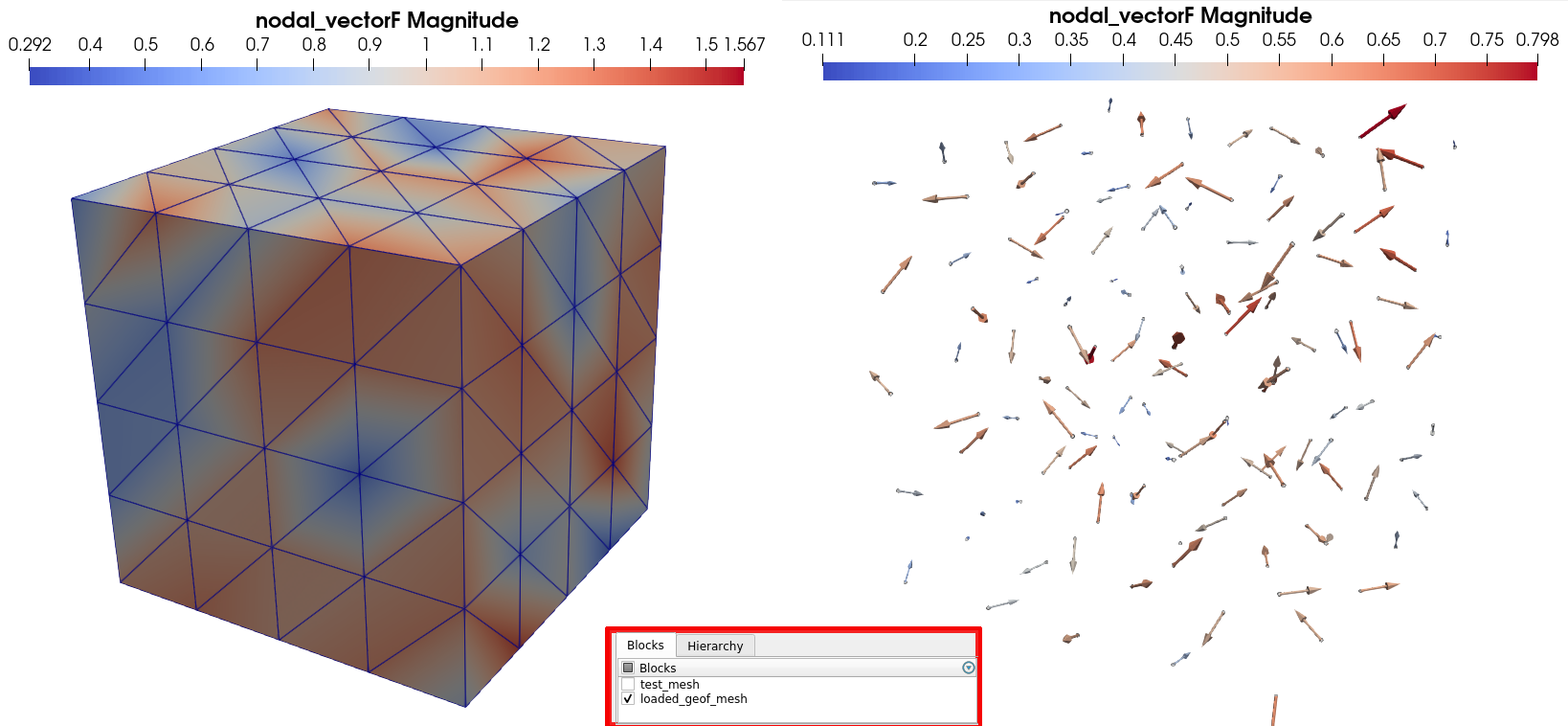
Open the XDMF dataset with the XdmfReader of Paraview, and then, in the Property panel, tick only the box associated to the the loaded_geof_mesh block. Then you can use the Glyph filter, which allows you to plot vector fields with arrows. You should be able to get visualization looking like the image below:
Example 2: Creating a scalar element field for boundary elements
Scalar fields defined on boundary can correspond for instance to pressure fields applied on a body, or a surface temperature measurement. They are also a common type of data for material mechanics datasets.
To add one, we need to create a 1D array (as the field is scalar) that has one value per boundary element in the mesh. in the present case, the mesh has as many bulk as boundary elements. To solve the ambiguity, the add field method has a bulk_padding argument. If it is True (default value), the field is padded as a bulk element field. If it is set to False, the field is padded as a boundary element field.
[45]:
# Random array creation. Warning ! 'Number_of_boundary_elements' attribute is a list !
array = np.random.rand(data.get_attribute('Number_of_boundary_elements','mesh_geof')[0])
# creation of the mesh field
data.add_field(gridname='mesh_geof', fieldname='boundary_scalarF', array=array, indexname='boundaryF', replace=True,
              bulk_padding=False)
[45]:
/loaded_geof_mesh/boundary_scalarF (CArray(768, 1)) 'boundaryF'
  atom := Float64Atom(shape=(), dflt=0.0)
  maindim := 0
  flavor := 'numpy'
  byteorder := 'little'
  chunkshape := (8192, 1)
[46]:
# Printing information on our created field:
print(f'Is "boundaryF" in the field list of the mesh ? {"boundaryF" in data.get_grid_field_list("mesh_geof")}')
data.print_node_info('boundaryF')
Is "boundaryF" in the field list of the mesh ? True

 NODE: /loaded_geof_mesh/boundary_scalarF
====================
 -- Parent Group : loaded_geof_mesh
 -- Node name : boundary_scalarF
 -- boundary_scalarF attributes :
         * empty : False
         * field_dimensionality : Scalar
         * field_type : Element_field
         * node_type : field_array
         * padding : boundary
         * parent_grid_path : /loaded_geof_mesh
         * xdmf_fieldname : boundary_scalarF
         * xdmf_gridname : loaded_geof_mesh

 -- content : /loaded_geof_mesh/boundary_scalarF (CArray(768, 1)) 'boundaryF'
 -- Compression options for node `boundaryF`:
        complevel=0, shuffle=False, bitshuffle=False, fletcher32=False, least_significant_digit=None
 --- Chunkshape: (8192, 1)
 -- Node memory size :    64.000 Kb
----------------
We can verify the field attributes to check that it is indeed a scalar element field, padded as a boundary element field, that is defined on the loaded_geof_mesh Mesh Group.
Once again, you can visualize your field with the Paraview software:
Open the XDMF dataset with the XdmfReader of Paraview, and then, in the Property panel, tick only the box associated to the the loaded_geof_mesh block. Then you can use the Clip filter, which allows you to cut your grid with a customizable plane and hence plot data within the bulk of your mesh, as the right picture below:
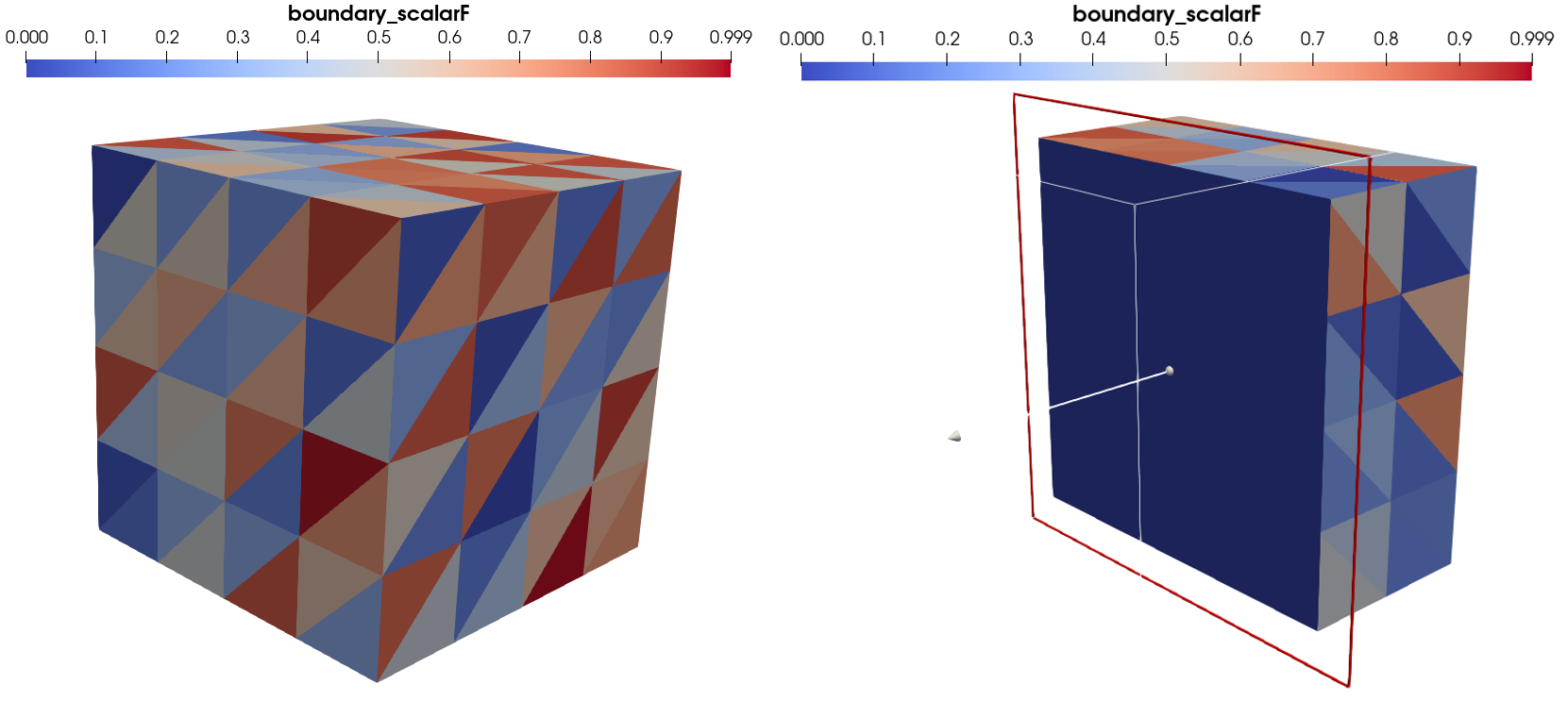
As you can see, the visual rendering of the field displays the random values of the field on the boundary triangle elements of the external surface of the mesh, and 0 values within the bulk of the mesh: SampleData has automatically padded the field array with 0 at positions corresponding to bulk elements to ensure compatibility with the XDMF format, and hence visualization.
Example 3: Creating a time serie for a tensorial integration point field for bulk elements
In this last example, we will add a field representing a uniaxial stress state to the mesh, proportional to time. We need to create a symetric tensor field, with 6 components. We will suppose that this field comes from a finite element solver output, that provided the full stress tensor at each integration point in the mesh bulk elements. We will suppose that the mesh elements have 4 integration points each, and that the values have been outputed at three instants.
Hence, we have to create 3 arrays of shape \((4N_{be},6)\), where \(N_{be}\) is the number of bulk elements in the mesh.
[47]:
# Arrays creation
array_T0 = np.zeros((4*data.get_attribute('Number_of_bulk_elements','mesh_geof')[0],6))
array_T1 = np.zeros((4*data.get_attribute('Number_of_bulk_elements','mesh_geof')[0],6))
array_T2 = np.zeros((4*data.get_attribute('Number_of_bulk_elements','mesh_geof')[0],6))

# time values:
T0 = 0.
T1 = 1.
T2 = 10.

# Filling stress state values
# at second time increment --> stress = 100*t in direction Z/3 (see indexing conventions)
array_T1[:,2] = 100*T1
# at second time increment --> stress = 100*t in direction Z/3 (see indexing conventions)
array_T2[:,2] = 100*T2

# create fields
data.add_field(gridname='mesh_geof', fieldname='tensor_ipF', array=array_T0, indexname='tensorF', replace=True,
              time=T0)
data.add_field(gridname='mesh_geof', fieldname='tensor_ipF', array=array_T1, indexname='tensorF', replace=True,
              time=T1)
data.add_field(gridname='mesh_geof', fieldname='tensor_ipF', array=array_T2, indexname='tensorF', replace=True,
              time=T2)
[47]:
/loaded_geof_mesh/tensor_ipF_T2 (CArray(1536, 6)) 'tensorF_T2'
  atom := Float64Atom(shape=(), dflt=0.0)
  maindim := 0
  flavor := 'numpy'
  byteorder := 'little'
  chunkshape := (1365, 6)
[48]:
print(data.get_grid_field_list('mesh_geof'))
data.print_node_info('tensorF_T0')
data.print_node_info('tensorF_T2')
['mesh_geof_field_x0y0z0', 'mesh_geof_field_x1y0z0', 'mesh_geof_field_x0y1z0', 'mesh_geof_field_x1y1z0', 'mesh_geof_field_x0y0z1', 'mesh_geof_field_x1y0z1', 'mesh_geof_field_x0y1z1', 'mesh_geof_field_x1y1z1', 'mesh_geof_field_3D', 'mesh_geof_field_X0', 'mesh_geof_field_Y0', 'mesh_geof_field_Skin', 'mesh_geof_field_X1', 'mesh_geof_field_Y1', 'mesh_geof_field_Z0', 'mesh_geof_field_Z1', 'vectF', 'boundaryF', 'tensorF_T0', 'tensorF_T1', 'tensorF_T2']

 NODE: /loaded_geof_mesh/tensor_ipF_T0
====================
 -- Parent Group : loaded_geof_mesh
 -- Node name : tensor_ipF_T0
 -- tensor_ipF_T0 attributes :
         * empty : False
         * field_dimensionality : Tensor6
         * field_type : IP_field
         * node_type : field_array
         * padding : bulk_IP
         * parent_grid_path : /loaded_geof_mesh
         * time : 0.0
         * time_serie_name : tensor_ipF
         * transpose_components : [0, 3, 5, 1, 4, 2]
         * visualisation_field_path : /loaded_geof_mesh/tensor_ipF_T0_Elt_mean
         * visualisation_type : Elt_mean
         * xdmf_gridname : loaded_geof_mesh_T0

 -- content : /loaded_geof_mesh/tensor_ipF_T0 (CArray(1536, 6)) 'tensorF_T0'
 -- Compression options for node `tensorF_T0`:
        complevel=0, shuffle=False, bitshuffle=False, fletcher32=False, least_significant_digit=None
 --- Chunkshape: (1365, 6)
 -- Node memory size :   127.969 Kb
----------------


 NODE: /loaded_geof_mesh/tensor_ipF_T2
====================
 -- Parent Group : loaded_geof_mesh
 -- Node name : tensor_ipF_T2
 -- tensor_ipF_T2 attributes :
         * empty : False
         * field_dimensionality : Tensor6
         * field_type : IP_field
         * node_type : field_array
         * padding : bulk_IP
         * parent_grid_path : /loaded_geof_mesh
         * time : 10.0
         * time_serie_name : tensor_ipF
         * transpose_components : [0, 3, 5, 1, 4, 2]
         * visualisation_field_path : /loaded_geof_mesh/tensor_ipF_T2_Elt_mean
         * visualisation_type : Elt_mean
         * xdmf_gridname : loaded_geof_mesh_T2

 -- content : /loaded_geof_mesh/tensor_ipF_T2 (CArray(1536, 6)) 'tensorF_T2'
 -- Compression options for node `tensorF_T2`:
        complevel=0, shuffle=False, bitshuffle=False, fletcher32=False, least_significant_digit=None
 --- Chunkshape: (1365, 6)
 -- Node memory size :   127.969 Kb
----------------
You can see that the fields have been automatically added as integration point fields symmetric tensor (Tensor6 IP_field). You can also observe the apparition of the transpose_components attribute, that has been already introduce in the last tutorial.
You can also observe that the fields have a visualisation_field_path and a visualisation_type attributes. They indicate respectively the path of the visualization field data item associated to our added field, as well as the type of operation that has been used to create it (here, taking the mean of integration points value within each element to create an element wise constant field: Elt_mean).
You can try to modify the calls to add_field in the previous cells by adding the visualisation_type argument, and setting its value to Elt_max, or None, and observe the differences in the field data item attributes, and the field visualization.
Let us now look at the XDMf dataset:
[49]:
data.print_xdmf()
<Xdmf xmlns:xi="http://www.w3.org/2003/XInclude" Version="2.2">
  <Domain>
    <Grid Name="test_mesh" GridType="Uniform">
      <Geometry Type="XYZ">
        <DataItem Format="HDF" Dimensions="6  3" NumberType="Float" Precision="64">test_mesh_dataset.h5:/test_mesh/Geometry/Nodes</DataItem>
      </Geometry>
      <Topology TopologyType="Triangle" NumberOfElements="8">
        <DataItem Format="HDF" Dimensions="24 " NumberType="Int" Precision="64">test_mesh_dataset.h5:/test_mesh/Geometry/Elements</DataItem>
      </Topology>
      <Attribute Name="field_Z0_plane" AttributeType="Scalar" Center="Node">
        <DataItem Format="HDF" Dimensions="6  1" NumberType="Int" Precision="8">test_mesh_dataset.h5:/test_mesh/Geometry/NodeTags/field_Z0_plane</DataItem>
      </Attribute>
      <Attribute Name="field_out_of_plane" AttributeType="Scalar" Center="Node">
        <DataItem Format="HDF" Dimensions="6  1" NumberType="Int" Precision="8">test_mesh_dataset.h5:/test_mesh/Geometry/NodeTags/field_out_of_plane</DataItem>
      </Attribute>
      <Attribute Name="field_2D" AttributeType="Scalar" Center="Cell">
        <DataItem Format="HDF" Dimensions="8  1" NumberType="Float" Precision="64">test_mesh_dataset.h5:/test_mesh/Geometry/ElementsTags/field_2D</DataItem>
      </Attribute>
      <Attribute Name="field_Top" AttributeType="Scalar" Center="Cell">
        <DataItem Format="HDF" Dimensions="8  1" NumberType="Float" Precision="64">test_mesh_dataset.h5:/test_mesh/Geometry/ElementsTags/field_Top</DataItem>
      </Attribute>
      <Attribute Name="field_Bottom" AttributeType="Scalar" Center="Cell">
        <DataItem Format="HDF" Dimensions="8  1" NumberType="Float" Precision="64">test_mesh_dataset.h5:/test_mesh/Geometry/ElementsTags/field_Bottom</DataItem>
      </Attribute>
      <Attribute Name="Test_field1" AttributeType="Scalar" Center="Node">
        <DataItem Format="HDF" Dimensions="6  1" NumberType="Float" Precision="64">test_mesh_dataset.h5:/test_mesh/Test_field1</DataItem>
      </Attribute>
      <Attribute Name="Test_field2" AttributeType="Scalar" Center="Node">
        <DataItem Format="HDF" Dimensions="6  1" NumberType="Float" Precision="64">test_mesh_dataset.h5:/test_mesh/Test_field2</DataItem>
      </Attribute>
      <Attribute Name="Test_field3" AttributeType="Scalar" Center="Cell">
        <DataItem Format="HDF" Dimensions="8  1" NumberType="Float" Precision="64">test_mesh_dataset.h5:/test_mesh/Test_field3</DataItem>
      </Attribute>
      <Attribute Name="Test_field4" AttributeType="Scalar" Center="Cell">
        <DataItem Format="HDF" Dimensions="8  1" NumberType="Float" Precision="64">test_mesh_dataset.h5:/test_mesh/Test_field4</DataItem>
      </Attribute>
    </Grid>
    <Grid Name="loaded_geof_mesh" GridType="Collection" CollectionType="Temporal">
      <Grid Name="loaded_geof_mesh_T0" GridType="Uniform">
        <Geometry Type="XYZ">
          <DataItem Format="HDF" Dimensions="125  3" NumberType="Float" Precision="64">test_mesh_dataset.h5:/loaded_geof_mesh/Geometry/Nodes</DataItem>
        </Geometry>
        <Topology TopologyType="Mixed" NumberOfElements="768">
          <DataItem Format="HDF" Dimensions="3456 " NumberType="Int" Precision="64">test_mesh_dataset.h5:/loaded_geof_mesh/Geometry/Elements</DataItem>
        </Topology>
        <Attribute Name="field_x0y0z0" AttributeType="Scalar" Center="Node">
          <DataItem Format="HDF" Dimensions="125  1" NumberType="Int" Precision="8">test_mesh_dataset.h5:/loaded_geof_mesh/Geometry/NodeTags/field_x0y0z0</DataItem>
        </Attribute>
        <Attribute Name="field_x1y0z0" AttributeType="Scalar" Center="Node">
          <DataItem Format="HDF" Dimensions="125  1" NumberType="Int" Precision="8">test_mesh_dataset.h5:/loaded_geof_mesh/Geometry/NodeTags/field_x1y0z0</DataItem>
        </Attribute>
        <Attribute Name="field_x0y1z0" AttributeType="Scalar" Center="Node">
          <DataItem Format="HDF" Dimensions="125  1" NumberType="Int" Precision="8">test_mesh_dataset.h5:/loaded_geof_mesh/Geometry/NodeTags/field_x0y1z0</DataItem>
        </Attribute>
        <Attribute Name="field_x1y1z0" AttributeType="Scalar" Center="Node">
          <DataItem Format="HDF" Dimensions="125  1" NumberType="Int" Precision="8">test_mesh_dataset.h5:/loaded_geof_mesh/Geometry/NodeTags/field_x1y1z0</DataItem>
        </Attribute>
        <Attribute Name="field_x0y0z1" AttributeType="Scalar" Center="Node">
          <DataItem Format="HDF" Dimensions="125  1" NumberType="Int" Precision="8">test_mesh_dataset.h5:/loaded_geof_mesh/Geometry/NodeTags/field_x0y0z1</DataItem>
        </Attribute>
        <Attribute Name="field_x1y0z1" AttributeType="Scalar" Center="Node">
          <DataItem Format="HDF" Dimensions="125  1" NumberType="Int" Precision="8">test_mesh_dataset.h5:/loaded_geof_mesh/Geometry/NodeTags/field_x1y0z1</DataItem>
        </Attribute>
        <Attribute Name="field_x0y1z1" AttributeType="Scalar" Center="Node">
          <DataItem Format="HDF" Dimensions="125  1" NumberType="Int" Precision="8">test_mesh_dataset.h5:/loaded_geof_mesh/Geometry/NodeTags/field_x0y1z1</DataItem>
        </Attribute>
        <Attribute Name="field_x1y1z1" AttributeType="Scalar" Center="Node">
          <DataItem Format="HDF" Dimensions="125  1" NumberType="Int" Precision="8">test_mesh_dataset.h5:/loaded_geof_mesh/Geometry/NodeTags/field_x1y1z1</DataItem>
        </Attribute>
        <Attribute Name="field_3D" AttributeType="Scalar" Center="Cell">
          <DataItem Format="HDF" Dimensions="768  1" NumberType="Int" Precision="8">test_mesh_dataset.h5:/loaded_geof_mesh/Geometry/ElementsTags/field_3D</DataItem>
        </Attribute>
        <Attribute Name="field_X0" AttributeType="Scalar" Center="Cell">
          <DataItem Format="HDF" Dimensions="768  1" NumberType="Int" Precision="8">test_mesh_dataset.h5:/loaded_geof_mesh/Geometry/ElementsTags/field_X0</DataItem>
        </Attribute>
        <Attribute Name="field_Y0" AttributeType="Scalar" Center="Cell">
          <DataItem Format="HDF" Dimensions="768  1" NumberType="Int" Precision="8">test_mesh_dataset.h5:/loaded_geof_mesh/Geometry/ElementsTags/field_Y0</DataItem>
        </Attribute>
        <Attribute Name="field_Skin" AttributeType="Scalar" Center="Cell">
          <DataItem Format="HDF" Dimensions="768  1" NumberType="Int" Precision="8">test_mesh_dataset.h5:/loaded_geof_mesh/Geometry/ElementsTags/field_Skin</DataItem>
        </Attribute>
        <Attribute Name="field_X1" AttributeType="Scalar" Center="Cell">
          <DataItem Format="HDF" Dimensions="768  1" NumberType="Int" Precision="8">test_mesh_dataset.h5:/loaded_geof_mesh/Geometry/ElementsTags/field_X1</DataItem>
        </Attribute>
        <Attribute Name="field_Y1" AttributeType="Scalar" Center="Cell">
          <DataItem Format="HDF" Dimensions="768  1" NumberType="Int" Precision="8">test_mesh_dataset.h5:/loaded_geof_mesh/Geometry/ElementsTags/field_Y1</DataItem>
        </Attribute>
        <Attribute Name="field_Z0" AttributeType="Scalar" Center="Cell">
          <DataItem Format="HDF" Dimensions="768  1" NumberType="Int" Precision="8">test_mesh_dataset.h5:/loaded_geof_mesh/Geometry/ElementsTags/field_Z0</DataItem>
        </Attribute>
        <Attribute Name="field_Z1" AttributeType="Scalar" Center="Cell">
          <DataItem Format="HDF" Dimensions="768  1" NumberType="Int" Precision="8">test_mesh_dataset.h5:/loaded_geof_mesh/Geometry/ElementsTags/field_Z1</DataItem>
        </Attribute>
        <Attribute Name="nodal_vectorF" AttributeType="Vector" Center="Node">
          <DataItem Format="HDF" Dimensions="125  3" NumberType="Float" Precision="64">test_mesh_dataset.h5:/loaded_geof_mesh/nodal_vectorF</DataItem>
        </Attribute>
        <Attribute Name="boundary_scalarF" AttributeType="Scalar" Center="Cell">
          <DataItem Format="HDF" Dimensions="768  1" NumberType="Float" Precision="64">test_mesh_dataset.h5:/loaded_geof_mesh/boundary_scalarF</DataItem>
        </Attribute>
        <Time Value="0.0"/>
        <Attribute Name="tensor_ipF" AttributeType="Tensor6" Center="Cell">
          <DataItem Format="HDF" Dimensions="768  6" NumberType="Float" Precision="64">test_mesh_dataset.h5:/loaded_geof_mesh/tensor_ipF_T0_Elt_mean</DataItem>
        </Attribute>
      </Grid>
      <Grid Name="loaded_geof_mesh_T1" GridType="Uniform">
        <Time Value="1.0"/>
        <Topology TopologyType="Mixed" NumberOfElements="768">
          <DataItem Format="HDF" Dimensions="3456 " NumberType="Int" Precision="64">test_mesh_dataset.h5:/loaded_geof_mesh/Geometry/Elements</DataItem>
        </Topology>
        <Geometry Type="XYZ">
          <DataItem Format="HDF" Dimensions="125  3" NumberType="Float" Precision="64">test_mesh_dataset.h5:/loaded_geof_mesh/Geometry/Nodes</DataItem>
        </Geometry>
        <Attribute Name="tensor_ipF" AttributeType="Tensor6" Center="Cell">
          <DataItem Format="HDF" Dimensions="768  6" NumberType="Float" Precision="64">test_mesh_dataset.h5:/loaded_geof_mesh/tensor_ipF_T1_Elt_mean</DataItem>
        </Attribute>
      </Grid>
      <Grid Name="loaded_geof_mesh_T2" GridType="Uniform">
        <Time Value="10.0"/>
        <Topology TopologyType="Mixed" NumberOfElements="768">
          <DataItem Format="HDF" Dimensions="3456 " NumberType="Int" Precision="64">test_mesh_dataset.h5:/loaded_geof_mesh/Geometry/Elements</DataItem>
        </Topology>
        <Geometry Type="XYZ">
          <DataItem Format="HDF" Dimensions="125  3" NumberType="Float" Precision="64">test_mesh_dataset.h5:/loaded_geof_mesh/Geometry/Nodes</DataItem>
        </Geometry>
        <Attribute Name="tensor_ipF" AttributeType="Tensor6" Center="Cell">
          <DataItem Format="HDF" Dimensions="768  6" NumberType="Float" Precision="64">test_mesh_dataset.h5:/loaded_geof_mesh/tensor_ipF_T2_Elt_mean</DataItem>
        </Attribute>
      </Grid>
    </Grid>
  </Domain>
</Xdmf>
As expected, the Attributes of our grid time collection loaded_geof_mesh that contain the tensor field do not point towards the added data array, but towards the visualization field data array: tensor_ipF_T0_Elt_mean, tensor_ipF_T1_Elt_mean or tensor_ipF_T2_Elt_mean.
VI - Getting Mesh Groups and Mesh Fields
Getting mesh objects from Mesh groups
Like Image groups, you can easily retrieve a complete SampleData Mesh Group under the form of a BasicTools Mesh object, with the get_mesh method:
[50]:
mesh = data.get_mesh('mesh_geof', with_fields=True, with_tags=True)
print(mesh)
UnstructuredMesh
  Number Of Nodes    : 125
    Tags : (x0y0z0:1) (x1y0z0:1) (x0y1z0:1) (x1y1z0:1) (x0y0z1:1) (x1y0z1:1) (x0y1z1:1) (x1y1z1:1)
  Number Of Elements : 768
    ElementsContainer,   Type : (tet4,384),   Tags : (3D:384)
    ElementsContainer,   Type : (tri3,384),   Tags : (X0:32) (Y0:32) (Skin:192) (X1:32) (Y1:32) (Z0:32) (Z1:32)
  nodeFields         : ['vectF']
  elemFields         : ['boundaryF']
This method has two arguments that allows you to control how rich you want your output to be. By setting with_fields to False, the return mesh object will not contain the field arrays stored on the Mesh Group. By setting with_tags to False, the return mesh object will not contain the Node and Element tags stored in the Mesh Group. If both are False, the mesh object will only contain the mesh nodes and elements.
Getting mesh Fields
As for image fields, retrieveing mesh fields from Sampledata dataset is done with the get_field method. All padding, transpositions etc… are automatically reverted to return the originally inputed data array.
In the case of mesh fields, you can prevent the reversion of field padding with the unpad_field argument (set it to False). You can also choose, when getting an integration point field, to get the complete data array, or on the contrary, only the associated visualization field data array, by setting the get_visualisation_field argument to True.
Let us show these various use of the method by trying to get the tensor field created in the third exampe above.
[51]:
# getting the inputed array --> no options
O_array = data.get_field('tensorF_T1')
# getting the visualization array
V_array = data.get_field('tensorF_T1', get_visualisation_field=True)
# getting the unpadded visualization array
UPV_array = data.get_field('tensorF_T1', unpad_field=False, get_visualisation_field=True)

print(f' Original array shape is {O_array.shape}, unpadded array shape is {V_array.shape},'
      f' unpadded visualization array shape is {UPV_array.shape}')

print(f'\nIs it the original inputed array ? {np.all(O_array == array_T1)} \n')
 Original array shape is (1536, 6), unpadded array shape is (384, 6), unpadded visualization array shape is (768, 6)

Is it the original inputed array ? True
As you can see, using get_field allow you to retrieve exactly the original array that you inputed, reverting all transformations (\(1536 = 4*384\) here). Using the get_visualisation_field argument, you retrieve the unpadded visualization field with values only for the mesh bulk elements, as inputted (\(384\) values here); and adding the unpad_field=False argument, you get the field with the added 0, that has one value per element in the mesh (\(768\) values here).
This is the end of this tutorial on SampleData Mesh Groups ! We can now close our dataset to conclude it.
[52]:
del data
SampleData Autodelete:
 Removing hdf5 file test_mesh_dataset.h5 and xdmf file test_mesh_dataset.xdmf