6 - Data Compression

This short Notebook will introduce you to how to efficiently compress your data within SampleData datasets.

Note

Throughout this notebook, it will be assumed that the reader is familiar with the overview of the SampleData file format and data model presented in the first notebook of this User Guide of this User Guide.

Data compression with HDF5 and Pytables

HDF5 and data compression

HDF5 allows compression filters to be applied to datasets in a file to minimize the amount of space it consumes. These compression features allow to drastically improve the storage space required for you datasets, as well as the speed of I/O access to datasets, and can differ from one data item to another within the same HDF5 file. A detailed presentation of HDF5 compression possibilities is provided here.

The two main ingredients that control compression performances for HDF5 datasets are the compression filters used (which compression algorithm, with which parameters), and the using a chunked layout for the data. This two features are briefly developed hereafter.

Pytables and data compression

The application of compression filters to HDF5 files with the SampleData class is handled by the Pytable package, on which is built the SampleData HDF5 interface. Pytables implements a specific containers class, the Filters class, to gather the various settings of the compression filters to apply to the datasets in a HDF5 file.

When using the SampleData class, you will have to specify this compression filter settings to class methods dedicated to data compression. These settings are the parameters of the Pytables Filters class. These settings and their possible values are detailed in the next subsection.

Available filter settings

The description given below of compression options available with SampleData/Pytables is exctracted from the *Pytables* documentation of the *Filter* class.

• complevel (int) – Specifies a compression level for data. The allowed range is 0-9. A value of 0 (the default) disables compression.

• complib (str) – Specifies the compression library to be used. Right now, zlib (the default), lzo, bzip2 and blosc are supported. Additional compressors for Blosc like blosc:blosclz (‘blosclz’ is the default in case the additional compressor is not specified), blosc:lz4, blosc:lz4hc, blosc:snappy, blosc:zlib and blosc:zstd are supported too. Specifying a compression library which is not available in the system issues a FiltersWarning and sets the library to the default one.

• shuffle (bool) – Whether or not to use the Shuffle filter in the HDF5 library. This is normally used to improve the compression ratio. A false value disables shuffling and a true one enables it. The default value depends on whether compression is enabled or not; if compression is enabled, shuffling defaults to be enabled, else shuffling is disabled. Shuffling can only be used when compression is enabled.

• bitshuffle (bool) – Whether or not to use the BitShuffle filter in the Blosc library. This is normally used to improve the compression ratio. A false value disables bitshuffling and a true one enables it. The default value is disabled.

• fletcher32 (bool) – Whether or not to use the Fletcher32 filter in the HDF5 library. This is used to add a checksum on each data chunk. A false value (the default) disables the checksum.

• least_significant_digit (int) – If specified, data will be truncated (quantized). In conjunction with enabling compression, this produces ‘lossy’, but significantly more efficient compression. For example, if least_significant_digit=1, data will be quantized using around(scale*data)/scale, where scale = 2^bits, and bits is determined so that a precision of 0.1 is retained (in this case bits=4). Default is None, or no quantization.

Chunked storage layout

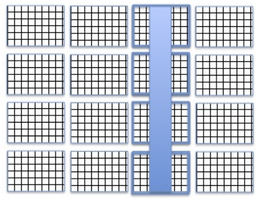
Compressed data is stored in a data array of an HDF5 dataset using a chunked storage mechanism. When chunked storage is used, the data array is split into equally sized chunks each of which is stored separately in the file, as illustred on the diagram below. Compression is applied to each individual chunk. When an I/O operation is performed on a subset of the data array, only chunks that include data from the subset participate in I/O and need to be uncompressed or compressed.

Chunking data allows to:

• Generally improve, sometimes drastically, the I/O performance of datasets. This comes from the fact that the chunked layout removes the reading speed anisotropy for data array that depends along which dimension its elements are read (i.e the same number of disk access are required when reading data in rows or columns).

• Chunked storage also enables adding more data to a dataset without rewriting the whole dataset.

By default, data arrays are stored with a chunked layout in SampleData datasets. The size of chunks is the key parameter that controls the impact on I/O performances for chunked datasets. The shape of chunks is computed automatically by the Pytable package, providing a value yielding generally good I/O performances. if you need to go further in the I/O optimization, you may consult the Pytables documentation page dedicated to compression optimization for I/O speed and storage space. In addition, it is highly recommended to read this document in order to be able to efficiently optimize I/O and storage performances for your chunked datasets. These performance issues will not be discussed in this tutorial.

Compressing your datasets with SampleData

Within Sampledata, data compression can be applied to:

• data arrays

• structured data arrays

• field data arrays

There are two ways to control the compression settings of your SampleData data arrays:

1. Providing compression settings to data item creation methods

2. Using the set_chunkshape_and_compression and set_nodes_compression_chunkshape methods

The compression options dictionary

In both cases, you will have to pass the various settings of the compression filter you want to apply to your data to the appropriate SampleData method. All of these methods accept for that purpose a compression_options argument, which must be a dictionary. Its keys and associated values can be chosen among the ones listed in the Available filter settings subsection above.

Compress already existing data arrays

We will start by looking at how we can change compression settings of already existing data in SampleData datasets. For that, we will use a material science dataset that is part of the Pymicro example datasets.

from config import PYMICRO_EXAMPLES_DATA_DIR # import file directory path
import os
dataset_file = os.path.join(PYMICRO_EXAMPLES_DATA_DIR, 'example_microstructure') # test dataset file path
tar_file = os.path.join(PYMICRO_EXAMPLES_DATA_DIR, 'example_microstructure.tar.gz') # dataset archive path

This file is zipped in the package to reduce its size. We will have to unzip it to use it and learn how to reduce its size with the SampleData methods. If you are just reading the documentation and not executing it, you may just skip this cell and the next one.

# Save current directory
cwd = os.getcwd()
# move to example data directory
os.chdir(PYMICRO_EXAMPLES_DATA_DIR)
# unarchive the dataset
os.system(f'tar -xvf {tar_file}')
# get back to UserGuide directory
os.chdir(cwd)

Dataset presentation

In this tutorial, we will work on a copy of this dataset, to leave the original data unaltered. We will start by creating an autodeleting copy of the file, and print its content to discover its content.

# import SampleData class
from pymicro.core.samples import SampleData as SD
# import Numpy
import numpy as np

# Create a copy of the existing dataset
data = SD.copy_sample(src_sample_file=dataset_file, dst_sample_file='Test_compression', autodelete=True,
                      get_object=True, overwrite=True)

print(data)
data.get_file_disk_size()

Dataset Content Index :
------------------------:
index printed with max depth `3` and under local root `/`

         Name : GrainDataTable                            H5_Path : /GrainData/GrainDataTable
         Name : Grain_data                                H5_Path : /GrainData
         Name : Image_data                                H5_Path : /CellData
                Image_data aliases --> `CellData`
         Name : Image_data_Amitex_stress_1                H5_Path : /CellData/Amitex_output_fields/Amitex_stress_1
         Name : Image_data_grain_map                      H5_Path : /CellData/grain_map
         Name : Image_data_grain_map_raw                  H5_Path : /CellData/grain_map_raw
         Name : Image_data_mask                           H5_Path : /CellData/mask
         Name : Image_data_uncertainty_map                H5_Path : /CellData/uncertainty_map
         Name : Mesh_data                                 H5_Path : /MeshData
         Name : Phase_data                                H5_Path : /PhaseData
         Name : fft_fields                                H5_Path : /CellData/Amitex_output_fields
         Name : fft_sim                                   H5_Path : /Amitex_Results
         Name : grain_map                                 H5_Path : /CellData/grain_map
         Name : grains_mesh                               H5_Path : /MeshData/grains_mesh
         Name : grains_mesh_Geometry                      H5_Path : /MeshData/grains_mesh/Geometry
         Name : grains_mesh_grains_mesh_elset_ids         H5_Path : /MeshData/grains_mesh/grains_mesh_elset_ids
         Name : mask                                      H5_Path : /CellData/mask
         Name : mean_strain                               H5_Path : /Amitex_Results/mean_strain
         Name : mean_stress                               H5_Path : /Amitex_Results/mean_stress
         Name : phase_01                                  H5_Path : /PhaseData/phase_01
         Name : phase_map                                 H5_Path : /CellData/phase_map
         Name : rms_strain                                H5_Path : /Amitex_Results/rms_strain
         Name : rms_stress                                H5_Path : /Amitex_Results/rms_stress
         Name : simulation_iterations                     H5_Path : /Amitex_Results/simulation_iterations
         Name : simulation_time                           H5_Path : /Amitex_Results/simulation_time

Printing dataset content with max depth 3
  |--GROUP Amitex_Results: /Amitex_Results (Group)
     --NODE mean_strain: /Amitex_Results/mean_strain (data_array) (   63.984 Kb)
     --NODE mean_stress: /Amitex_Results/mean_stress (data_array) (   63.984 Kb)
     --NODE rms_strain: /Amitex_Results/rms_strain (data_array) (   63.984 Kb)
     --NODE rms_stress: /Amitex_Results/rms_stress (data_array) (   63.984 Kb)
     --NODE simulation_iterations: /Amitex_Results/simulation_iterations (data_array) (   64.000 Kb)
     --NODE simulation_time: /Amitex_Results/simulation_time (data_array) (   64.000 Kb)

  |--GROUP CellData: /CellData (3DImage)
    |--GROUP Amitex_output_fields: /CellData/Amitex_output_fields (Group)
       --NODE Amitex_stress_1: /CellData/Amitex_output_fields/Amitex_stress_1 (field_array) (   49.438 Mb)

     --NODE Field_index: /CellData/Field_index (string_array) (   63.999 Kb)
     --NODE grain_map: /CellData/grain_map (field_array) (    1.945 Mb)
     --NODE grain_map_raw: /CellData/grain_map_raw (field_array) (    1.945 Mb)
     --NODE mask: /CellData/mask (field_array) (  996.094 Kb)
     --NODE phase_map: /CellData/phase_map (field_array - empty) (   64.000 Kb)
     --NODE uncertainty_map: /CellData/uncertainty_map (field_array) (  996.094 Kb)

  |--GROUP GrainData: /GrainData (Group)
     --NODE GrainDataTable: /GrainData/GrainDataTable (structured array) (   63.984 Kb)

  |--GROUP MeshData: /MeshData (emptyMesh)
    |--GROUP grains_mesh: /MeshData/grains_mesh (3DMesh)
      |--GROUP Geometry: /MeshData/grains_mesh/Geometry (Group)
       --NODE grains_mesh_elset_ids: /MeshData/grains_mesh/grains_mesh_elset_ids (field_array) (  624.343 Kb)


  |--GROUP PhaseData: /PhaseData (Group)
    |--GROUP phase_01: /PhaseData/phase_01 (Group)


File size is    83.086 Mb for file
 Test_compression.h5

(83.08567428588867, 'Mb')

As you can see, this dataset already contains a rich content. It is a digital twin of a real polycristalline microstructure of a grade 2 Titanium sample, gathering both experimental and numerical data obtained through Diffraction Contrast Tomography imaging, and FFT-based mechanical simulation.

This dataset has actually been constructed using the Microstructure class of the pymicro package, which is based on the SampleData class. The link between these classes will be discussed in the next tutorial.

This dataset contains only uncompressed data. We will try to reduce its size by using various compression methods on the large data items that it contains. You can see that most of them are stored in the 3DImage Group CellData.

Apply compression settings for a specific array

We will start by compressing the grain_map Field data array of the CellData image. Let us look more closely on this data item:

data.print_node_info('grain_map')

 NODE: /CellData/grain_map
====================
 -- Parent Group : CellData
 -- Node name : grain_map
 -- grain_map attributes :
         * empty : False
         * field_dimensionality : Scalar
         * field_type : Element_field
         * node_type : field_array
         * padding : None
         * parent_grid_path : /CellData
         * transpose_indices : [2, 1, 0]
         * xdmf_fieldname : grain_map
         * xdmf_gridname : CellData

 -- content : /CellData/grain_map (CArray(100, 100, 100)) 'Image_data_grain_map'
 -- Compression options for node `grain_map`:
        complevel=0, shuffle=False, bitshuffle=False, fletcher32=False, least_significant_digit=None
 --- Chunkshape: (3, 100, 100)
 -- Node memory size :     1.945 Mb
----------------

We can see above that this data item is not compressed (complevel=0), and has a disk size of almost 2 Mb.

To apply a set of compression settings to this data item, you need to:

1. create a dictionary specifying the compression settings:

compression_options = {'complib':'zlib', 'complevel':1}

2. use the SampleData set_chunkshape_and_compression method with the dictionary and the name of the data item as arguments

data.set_chunkshape_and_compression(nodename='grain_map', compression_options=compression_options)
data.get_node_disk_size('grain_map')
data.print_node_compression_info('grain_map')

Node grain_map size on disk is   126.297 Kb
Compression options for node `grain_map`:
        complevel=1, complib='zlib', shuffle=False, bitshuffle=False, fletcher32=False, least_significant_digit=None
 --- Chunkshape: (3, 100, 100)

As you can see, the storage size of the data item has been greatly reduced, by more than 10 times (126 Kb vs 1.945 Mb), using this compression settings. Let us see what will change if we use different settings :

# No `shuffle` option:
print('\nUsing the shuffle option, with the zlib compressor and a compression level of 1:')
compression_options = {'complib':'zlib', 'complevel':1, 'shuffle':True}
data.set_chunkshape_and_compression(nodename='grain_map', compression_options=compression_options)
data.get_node_disk_size('grain_map')

# No `shuffle` option:
print('\nUsing no shuffle option, with the zlib compressor and a compression level of 9:')
compression_options = {'complib':'zlib', 'complevel':9, 'shuffle':False}
data.set_chunkshape_and_compression(nodename='grain_map', compression_options=compression_options)
data.get_node_disk_size('grain_map')

# No `shuffle` option:
print('\nUsing the shuffle option, with the lzo compressor and a compression level of 1:')
compression_options = {'complib':'lzo', 'complevel':1, 'shuffle':True}
data.set_chunkshape_and_compression(nodename='grain_map', compression_options=compression_options)
data.get_node_disk_size('grain_map')

# No `shuffle` option:
print('\nUsing no shuffle option, with the lzo compressor and a compression level of 1:')
compression_options = {'complib':'lzo', 'complevel':1, 'shuffle':False}
data.set_chunkshape_and_compression(nodename='grain_map', compression_options=compression_options)
data.get_node_disk_size('grain_map')

Using the shuffle option, with the zlib compressor and a compression level of 1:

Node grain_map size on disk is   179.201 Kb

Using no shuffle option, with the zlib compressor and a compression level of 9:

Node grain_map size on disk is    62.322 Kb

Using the shuffle option, with the lzo compressor and a compression level of 1:

Node grain_map size on disk is   327.034 Kb

Using no shuffle option, with the lzo compressor and a compression level of 1:

Node grain_map size on disk is   238.415 Kb

(238.4150390625, 'Kb')

As you may observe, is significantly affected by the choice of the compression level. The higher the compression level, the higher the compression ratio, but also the lower the I/O speed. On the other hand, you can also remark that, in the present case, using the shuffle filter deteriorates the compression ratio.

Let us try to with another data item:

data.print_node_info('Amitex_stress_1')

# No `shuffle` option:
print('\nUsing the shuffle option, with the zlib compressor and a compression level of 1:')
compression_options = {'complib':'zlib', 'complevel':1, 'shuffle':True}
data.set_chunkshape_and_compression(nodename='Amitex_stress_1', compression_options=compression_options)
data.get_node_disk_size('Amitex_stress_1')

# No `shuffle` option:
print('\nUsing no shuffle option, with the zlib compressor and a compression level of 1:')
compression_options = {'complib':'zlib', 'complevel':1, 'shuffle':False}
data.set_chunkshape_and_compression(nodename='Amitex_stress_1', compression_options=compression_options)
data.get_node_disk_size('Amitex_stress_1')

 NODE: /CellData/Amitex_output_fields/Amitex_stress_1
====================
 -- Parent Group : Amitex_output_fields
 -- Node name : Amitex_stress_1
 -- Amitex_stress_1 attributes :
         * empty : False
         * field_dimensionality : Tensor6
         * field_type : Element_field
         * node_type : field_array
         * padding : None
         * parent_grid_path : /CellData
         * transpose_components : [0, 3, 5, 1, 4, 2]
         * transpose_indices : [2, 1, 0, 3]
         * xdmf_fieldname : Amitex_stress_1
         * xdmf_gridname : CellData

 -- content : /CellData/Amitex_output_fields/Amitex_stress_1 (CArray(100, 100, 100, 6)) 'Image_data_Amitex_stress_1'
 -- Compression options for node `Amitex_stress_1`:
        complevel=0, shuffle=False, bitshuffle=False, fletcher32=False, least_significant_digit=None
 --- Chunkshape: (1, 27, 100, 6)
 -- Node memory size :    49.438 Mb
----------------



Using the shuffle option, with the zlib compressor and a compression level of 1:

Node Amitex_stress_1 size on disk is    20.975 Mb

Using no shuffle option, with the zlib compressor and a compression level of 1:

Node Amitex_stress_1 size on disk is    27.460 Mb

(27.460082054138184, 'Mb')

On the opposite, for this second array, the shuffle filter improves significantly the compression ratio. However, in this case, you can see that the compression ratio achieved is much lower than for the grain_map array.

Warning 1

The efficiency of compression algorithms in terms of compression ratio is strongly affected by the data itself (variety, value and position of the stored values in the array). Compression filters will not have the same behavior with all data arrays, as you have observed just above. Be aware of this fact, and do not hesitate to conduct tests to find the best settings for you datasets !

Warning 2

Whenever you change the compression or chunkshape settings of your datasets, the data item is re-created into the SampleData dataset, which may be costly in computational time. Be careful if you are dealing with very large data arrays and want to try out several settings to find the best I/O speed / compression ratio compromise, with the set_chunkshape_and_compression method. You may want to try on a subset of your large array to speed up the process.

Apply same compression settings for a serie of nodes

If you need to apply the same compression settings to a list of data items, you may use the set_nodes_compression_chunkshape. This method works exactly like set_chunkshape_and_compression, but take a list of nodenames as arguments instead of just one. The inputted compression settings are then applied to all the nodes in the list:

# Print current size of disks and their compression settings
data.get_node_disk_size('grain_map_raw')
data.print_node_compression_info('grain_map_raw')
data.get_node_disk_size('uncertainty_map')
data.print_node_compression_info('uncertainty_map')
data.get_node_disk_size('mask')
data.print_node_compression_info('mask')

# Compress datasets
compression_options = {'complib':'zlib', 'complevel':9, 'shuffle':True}
data.set_nodes_compression_chunkshape(node_list=['grain_map_raw', 'uncertainty_map', 'mask'],
                                      compression_options=compression_options)

# Print new size of disks and their compression settings
data.get_node_disk_size('grain_map_raw')
data.print_node_compression_info('grain_map_raw')
data.get_node_disk_size('uncertainty_map')
data.print_node_compression_info('uncertainty_map')
data.get_node_disk_size('mask')
data.print_node_compression_info('mask')

Node grain_map_raw size on disk is     1.945 Mb
Compression options for node `grain_map_raw`:
        complevel=0, shuffle=False, bitshuffle=False, fletcher32=False, least_significant_digit=None
 --- Chunkshape: (3, 100, 100)
Node uncertainty_map size on disk is   996.094 Kb
Compression options for node `uncertainty_map`:
        complevel=0, shuffle=False, bitshuffle=False, fletcher32=False, least_significant_digit=None
 --- Chunkshape: (6, 100, 100)
Node mask size on disk is   996.094 Kb
Compression options for node `mask`:
        complevel=0, shuffle=False, bitshuffle=False, fletcher32=False, least_significant_digit=None
 --- Chunkshape: (6, 100, 100)



Node grain_map_raw size on disk is   134.527 Kb
Compression options for node `grain_map_raw`:
        complevel=9, complib='zlib', shuffle=True, bitshuffle=False, fletcher32=False, least_significant_digit=None
 --- Chunkshape: (3, 100, 100)
Node uncertainty_map size on disk is    55.322 Kb
Compression options for node `uncertainty_map`:
        complevel=9, complib='zlib', shuffle=True, bitshuffle=False, fletcher32=False, least_significant_digit=None
 --- Chunkshape: (6, 100, 100)
Node mask size on disk is     1.363 Kb
Compression options for node `mask`:
        complevel=9, complib='zlib', shuffle=True, bitshuffle=False, fletcher32=False, least_significant_digit=None
 --- Chunkshape: (6, 100, 100)

Lossy compression and data normalization

The compression filters used above preserve exactly the original values of the stored data. However, it is also possible with specific filters a lossy compression, which remove non relevant part of the data. As a result, data compression ratio is usually strongly increased, at the cost that stored data is no longer exactly equal to the inputed data array.

One of the most important feature of data array that increase their compressibility, is the presence of patterns in the data. If a value or a serie of values is repeated multiple times throughout the data array, data compression can be very efficient (the pattern can be stored only once).

Numerical simulation and measurement tools usually output data in a standard simple or double precision floating point numbers, yiedling data arrays with values that have a lot of digits. Typically, these values are all different, and hence these arrays cannot be efficiently compressed.

The Amitex_stress_1 and Amitex_strain_1 data array are two tensor fields outputed by a continuum mechanics FFT-based solver, and typical fall into this category: they have almost no equal value or clear data pattern.

As you can see above, the best achieved compression ratio is 60% while for the dataset grain_map, the compression is way more efficient, with a best ratio that climbs up to 97% (62 Kb with zlib compressor and compression level of 9, versus an initial data array of 1.945 Mb). This is due to the nature of the grain_map data array, which is a tridimensional map of grains identification number in microstructure of the Titanium sample represented by the dataset. It is hence an array containing a few integer values that are repeated many times.

Let us analyze these two data arrays values to illustrate this difference:

import numpy as np
print(f"Data array `grain_map` has {data['grain_map'].size} elements,"
      f"and {np.unique(data['grain_map']).size} different values.\n")
print(f"Data array `Amitex_stress_1` has {data['Amitex_stress_1'].size} elements,"
      f"and {np.unique(data['Amitex_stress_1']).size} different values.\n")

Data array `grain_map` has 1000000 elements,and 111 different values.

Data array `Amitex_stress_1` has 6000000 elements,and 5443754 different values.

Lossy compression

Usually, the relevant precision of data is only of a few digits, so that many values of the array should be considered equal. The idea of lossy compression is to truncate values up to a desired precision, which increases the number of equal values in a dataset and hence increases its compressibility.

Lossy compression can be applied to floating point data arrays in SampleData datasets using the least_significant_digit compression setting. If you set the value of this option to \(N\), the data will be truncated after the \(N^{th}\) siginificant digit after the decimal point. Let us see an example.

# We will store a value of an array to verify how it evolves after compression
original_value = data['Amitex_stress_1'][20,20,20]

# Apply lossy compression
data.get_node_disk_size('Amitex_stress_1')
# Set up compression settings with lossy compression: truncate after third digit adter decimal point
compression_options = {'complib':'zlib', 'complevel':9, 'shuffle':True,  'least_significant_digit':3}
data.set_chunkshape_and_compression(nodename='Amitex_stress_1', compression_options=compression_options)
data.get_node_disk_size('Amitex_stress_1')

# Get same value after lossy compression
new_value = data['Amitex_stress_1'][20,20,20]

print(f'Original array value: {original_value} \n'
      f'Array value after lossy compression: {new_value}')

Node Amitex_stress_1 size on disk is    27.460 Mb

Node Amitex_stress_1 size on disk is    15.253 Mb
Original array value: [ -27.8652935   -48.22042084 1063.31445312   11.1795702   -21.17892647
   49.37730026]
Array value after lossy compression: [ -27.86523438  -48.22070312 1063.31445312   11.1796875   -21.17871094
   49.37695312]

As you may observe, the compression ratio has been improved, and the retrieved values after lossy compression are effectively equal to the original array up to the third digit after the decimal point.

We will now try to increase the compression ratio by reducing the number of conserved digits to 2:

# Set up compression settings with lossy compression: truncate after third digit adter decimal point
compression_options = {'complib':'zlib', 'complevel':9, 'shuffle':True,  'least_significant_digit':2}
data.set_chunkshape_and_compression(nodename='Amitex_stress_1', compression_options=compression_options)
data.get_node_disk_size('Amitex_stress_1')

# Get same value after lossy compression
new_value = data['Amitex_stress_1'][20,20,20]

print(f'Original array value: {original_value} \n'
      f'Array value after lossy compression 2 digits: {new_value}')

Node Amitex_stress_1 size on disk is    12.562 Mb
Original array value: [ -27.8652935   -48.22042084 1063.31445312   11.1795702   -21.17892647
   49.37730026]
Array value after lossy compression 2 digits: [ -27.8671875  -48.21875   1063.3125      11.1796875  -21.1796875
   49.375    ]

As you can see, the compression ratio has again been improved, now close to 75%. Know, you know how to do to choose the best compromise between lost precision and compression ratio.

Normalization to improve compression ratio

If you look more closely to the Amitex_stress_1 array values, you can observe that the value of this array have been outputed within a certain scale of values, which in particular impact the number of significant digits that come before the decimal point. Sometimes precision of the data would require less significant digits than its scale of representation.

In that case, storing the complete data array at its original scale is not necessary, and very inefficient in terms of data size. To optimize storage of such datasets, one can normalize them to a form with very few digits before the decimal point (1 or 2), and stored separately their scale to be able to revert the normalization operation when retrieiving data.

This allows to reduce the total number of significant digits of the data, and hence further improve the achievable compression ratio with lossy compression.

The SampleData class allows you to aplly automatically this operation when applying compression settings to your dataset. All you have to do is add to the compression_option dictionary the key normalization with one of its possible values.

To try it, we will close (and delete) our test dataset and recopy the original file, to apply normalization and lossy compression on the original raw data:

# removing dataset to recreate a copy
del data
# creating a copy of the dataset to try out lossy compression methods
data = SD.copy_sample(src_sample_file=dataset_file, dst_sample_file='Test_compression', autodelete=True,
                      get_object=True, overwrite=True)

SampleData Autodelete:
 Removing hdf5 file Test_compression.h5 and xdmf file Test_compression.xdmf

Standard Normalization

The standard normalization setting will center and reduce the data of an array \(X\) by storing a new array \(Y\) that is:

\(Y = \frac{X - \bar{X}}{\sigma(X)}\)

where \(\bar{X}\) and \(\sigma(X)\) are respectively the mean and the standard deviation of the data array \(X\).

This operation reduces the number of significant digits before the decimal point to 1 or 2 for the large majority of the data array values. After standard normalization, lossy compression will yield much higher compression ratios for data array that have a non normalized scale.

The SampleData class ensures that when data array are retrieved, or visualized, the user gets or sees the original data, with the normalization reverted.

Let us try to apply it to our stress field Amitex_stress_1.

# Set up compression settings with lossy compression: truncate after third digit adter decimal point
compression_options = {'complib':'zlib', 'complevel':9, 'shuffle':True,  'least_significant_digit':2,
                       'normalization':'standard'}
data.set_chunkshape_and_compression(nodename='Amitex_stress_1', compression_options=compression_options)
data.get_node_disk_size('Amitex_stress_1')

# Get same value after lossy compression
new_value = data['Amitex_stress_1'][20,20,20,:]

# Get in memory value of the node
memory_value = data.get_node('Amitex_stress_1', as_numpy=False)[20,20,20,:]

print(f'Original array value: {original_value} \n'
      f'Array value after normalization and lossy compression 2 digits: {new_value}',
      f'Value in memory: {memory_value}')

Node Amitex_stress_1 size on disk is     4.954 Mb
Original array value: [ -27.8652935   -48.22042084 1063.31445312   11.1795702   -21.17892647
   49.37730026]
Array value after normalization and lossy compression 2 digits: [ -27.50489858  -49.33973504 1064.23692429    9.92624963  -21.26637388
   50.47666019] Value in memory: [-0.515625  -0.421875  -0.3203125 -0.5703125 -0.5        2.21875  ]

As you can see, the compression ratio has been strongly improved by this normalization operation, reaching 90%. When looking at the retrieved value after compression, you can see that depending on the field component that is observed, the relative precision loss varies. The third large component value error is less than 1%, which is consistent with the truncation to 2 significant digits. However, it is not the other components, that have smaller values by two or three orders of magnitude, and that are retrieved with larger errors.

This is explained by the fact that the standard normalization option scales the array as a whole. As a result, if there are large differencies in the scale of different components of a vector or tensor field, the precision of the smaller components will be less preserved.

Standard Normalization per components for vector/tensor fields

Another normalization option is available for SampleData field arrays, that allows to apply standard normalization individually to each component of a field in order to keep a constant relative precision for each component when applying lossy compression to the field data array.

To use this option, you will need to set the normalization value to standard_per_component:

del data

SampleData Autodelete:
 Removing hdf5 file Test_compression.h5 and xdmf file Test_compression.xdmf

data = SD.copy_sample(src_sample_file=dataset_file, dst_sample_file='Test_compression', autodelete=True,
                      get_object=True, overwrite=True)

# Set up compression settings with lossy compression: truncate after third digit adter decimal point
compression_options = {'complib':'zlib', 'complevel':9, 'shuffle':True,  'least_significant_digit':2,
                       'normalization':'standard_per_component'}
data.set_chunkshape_and_compression(nodename='Amitex_stress_1', compression_options=compression_options)
data.get_node_disk_size('Amitex_stress_1')

# Get same value after lossy compression
new_value = data['Amitex_stress_1'][20,20,20,:]

# Get in memory value of the node
memory_value = data.get_node('Amitex_stress_1', as_numpy=False)[20,20,20,:]

print(f'Original array value: {original_value} \n'
      f'Array value after normalization per component and lossy compression 2 digits: {new_value}\n',
      f'Value in memory: {memory_value}')

Node Amitex_stress_1 size on disk is     8.117 Mb
Original array value: [ -27.8652935   -48.22042084 1063.31445312   11.1795702   -21.17892647
   49.37730026]
Array value after normalization per component and lossy compression 2 digits: [ -27.77213549  -48.1522771  1063.34782307   11.2637209   -21.14744986
   49.32227028]
 Value in memory: [-0.53125    0.484375   0.984375  -0.890625  -0.9453125 -0.0859375]

As you can see, the error in the retrieved array is now less than 1% for each component of the field value. However, the cost was a reduced improvement of the compression ratio.

Visualization of normalized data

data.print_xdmf()

<!DOCTYPE Xdmf SYSTEM "Xdmf.dtd">
<Xdmf xmlns:xi="http://www.w3.org/2003/XInclude" Version="2.2">
  <Domain>
    <Grid Name="CellData" GridType="Uniform">
      <Topology TopologyType="3DCoRectMesh" Dimensions="101 101 101"/>
      <Geometry Type="ORIGIN_DXDYDZ">
        <DataItem Format="XML" Dimensions="3">0. 0. 0.</DataItem>
        <DataItem Format="XML" Dimensions="3">0.00122 0.00122 0.00122</DataItem>
      </Geometry>
      <Attribute Name="grain_map" AttributeType="Scalar" Center="Cell">
        <DataItem Format="HDF" Dimensions="100  100  100" NumberType="Int" Precision="16">Test_compression.h5:/CellData/grain_map</DataItem>
      </Attribute>
      <Attribute Name="mask" AttributeType="Scalar" Center="Cell">
        <DataItem Format="HDF" Dimensions="100  100  100" NumberType="Int" Precision="uint8">Test_compression.h5:/CellData/mask</DataItem>
      </Attribute>
      <Attribute Name="grain_map_raw" AttributeType="Scalar" Center="Cell">
        <DataItem Format="HDF" Dimensions="100  100  100" NumberType="Int" Precision="16">Test_compression.h5:/CellData/grain_map_raw</DataItem>
      </Attribute>
      <Attribute Name="uncertainty_map" AttributeType="Scalar" Center="Cell">
        <DataItem Format="HDF" Dimensions="100  100  100" NumberType="Int" Precision="uint8">Test_compression.h5:/CellData/uncertainty_map</DataItem>
      </Attribute>
      <Attribute Name="Amitex_stress_1" AttributeType="Tensor6" Center="Cell">
        <DataItem ItemType="Function" Function="($2*$0) + $1" Dimensions="100  100  100  6">
          <DataItem Format="HDF" Dimensions="100  100  100  6" NumberType="Float" Precision="64">Test_compression.h5:/CellData/Amitex_output_fields/Amitex_stress_1</DataItem>
          <DataItem Format="HDF" Dimensions="100  100  100  6" NumberType="Float" Precision="64">Test_compression.h5:/CellData/Amitex_output_fields/Amitex_stress_1_norm_mean</DataItem>
          <DataItem Format="HDF" Dimensions="100  100  100  6" NumberType="Float" Precision="64">Test_compression.h5:/CellData/Amitex_output_fields/Amitex_stress_1_norm_std</DataItem>
        </DataItem>
      </Attribute>
    </Grid>
    <Grid Name="grains_mesh" GridType="Uniform">
      <Geometry Type="XYZ">
        <DataItem Format="HDF" Dimensions="92755  3" NumberType="Float" Precision="64">Test_compression.h5:/MeshData/grains_mesh/Geometry/Nodes</DataItem>
      </Geometry>
      <Topology TopologyType="Tetrahedron" NumberOfElements="490113">
        <DataItem Format="HDF" Dimensions="1960452 " NumberType="Int" Precision="64">Test_compression.h5:/MeshData/grains_mesh/Geometry/Elements</DataItem>
      </Topology>
      <Attribute Name="grains_mesh_elset_ids" AttributeType="Scalar" Center="Cell">
        <DataItem Format="HDF" Dimensions="490113  1" NumberType="Float" Precision="64">Test_compression.h5:/MeshData/grains_mesh/grains_mesh_elset_ids</DataItem>
      </Attribute>
    </Grid>
  </Domain>
</Xdmf>

As you can see, the Amitex_stress_1 Attribute node data in the dataset XDMF file is now provided by a Function item type, involving three data array with the original field shape. This function computes:

\(X' = Y*\sigma(X) + \bar{X}\)

where \(*\) and \(+\) are element-wise product and addition operators for multidimensional arrays. This operation allows to revert the component-wise normalization of data. The Paraview software is able to interpret this syntax of the XDMF format and hence, when visualizing data, you will see the values with the original scaling.

This operation required the creation of two large arrays in the dataset, that the store the mean and standard deviation of each component of the field, repeted for each spatial dimensions of the field data array. It is mandatory to allow visualization of the data with the right scaling in Paraview. However, as these array contain a very low amount of data (\(2*N_c\): two times de number of components of the field), they can be very easily compressed and hence do not significantly affect the storage size of the data item, as you may see below:

data.get_node_disk_size('Amitex_stress_1')
data.get_node_disk_size('Amitex_stress_1_norm_std')
data.get_node_disk_size('Amitex_stress_1_norm_mean')

Node Amitex_stress_1 size on disk is     8.117 Mb
Node Amitex_stress_1_norm_std size on disk is    75.781 Kb
Node Amitex_stress_1_norm_mean size on disk is    84.473 Kb

(84.47265625, 'Kb')

Changing the chunksize of a node

Compressing all fields when adding Image or Mesh Groups

Changing the chunksize of a data array with SampleData is very simple. You just have to pass as a tuple the news shape of the chunks you want for your data array, and pass it as an argument to the set_chunkshape_and_compression or set_nodes_compression_chunkshape:

data.print_node_compression_info('Amitex_stress_1')
data.get_node_disk_size('Amitex_stress_1')

Compression options for node `Amitex_stress_1`:
        complevel=9, complib='zlib', shuffle=True, bitshuffle=False, fletcher32=False, least_significant_digit=None
 --- Chunkshape: (1, 27, 100, 6)
Node Amitex_stress_1 size on disk is     8.117 Mb

(8.117431640625, 'Mb')

# Change chunkshape of the array
compression_options = {'complib':'zlib', 'complevel':9, 'shuffle':True,  'least_significant_digit':2,
                       'normalization':'standard_per_component'}
data.set_chunkshape_and_compression(nodename='Amitex_stress_1', chunkshape=(10,10,10,6),
                                   compression_options=compression_options)
data.get_node_disk_size('Amitex_stress_1')
data.print_node_compression_info('Amitex_stress_1')

Node Amitex_stress_1 size on disk is     7.950 Mb
Compression options for node `Amitex_stress_1`:
        complevel=9, complib='zlib', shuffle=True, bitshuffle=False, fletcher32=False, least_significant_digit=None
 --- Chunkshape: (10, 10, 10, 6)

As you can see, the chunkshape has been changed, which has also affected the memory size of the compressed data array. We have indeed reduced the number of chunks in the dataset, which reduces the number of data to store. This modification can also improve or deteriorate the I/O speed of access to your data array in the dataset. The reader is once again refered to dedicated documents to know more ion this matter: here and here.

Compression data and setting chunkshape upon creation of data items

Until here we have only modified the compression settings of already existing data items. In this process, the data items are replaced by the new compressed version of the data, which is a costly operation. For this reason, if they are known in advance, it is best to apply the compression filters and appropriate chunkshape when creating the data item.

If you have read through all the tutorials of this user guide, you should know all the method that allow to create data items in your datasets, like add_data_array, add_field, ædd_mesh… All of these methods accept the two arguments chunkshape and compression_options, that work exaclty as for the set_chunkshape_and_compression or set_nodes_compression_chunkshape methods. You hence use them to create your data items directly with the appropriate compression settings.

Let us see an example. We will get an array from our dataset, and try to recreate it with a new name and some data compression:

# removing dataset to recreate a copy
del data
# creating a copy of the dataset to try out lossy compression methods
data = SD.copy_sample(src_sample_file=dataset_file, dst_sample_file='Test_compression', autodelete=True,
                      get_object=True, overwrite=True)

SampleData Autodelete:
 Removing hdf5 file Test_compression.h5 and xdmf file Test_compression.xdmf

# getting the `orientation_map` array
array = data['Amitex_stress_1']

# create a new field for the CellData image group with the `orientation_map` array and add compression settings
compression_options = {'complib':'zlib', 'complevel':1, 'shuffle':True,  'least_significant_digit':2,
                       'normalization':'standard'}
new_cshape = (10,10,10,3)

# Add data array as field of the CellData Image Group
data.add_field(gridname='CellData', fieldname='test_compression', indexname='testC', array=array,
              chunkshape=new_cshape, compression_options=compression_options, replace=True)

/CellData/test_compression (CArray(100, 100, 100, 6), shuffle, zlib(1)) 'testC'
  atom := Float64Atom(shape=(), dflt=0.0)
  maindim := 0
  flavor := 'numpy'
  byteorder := 'little'
  chunkshape := (10, 10, 10, 3)

# Check size and settings of new field
data.print_node_info('testC')
data.get_node_disk_size('testC')
data.print_node_compression_info('testC')

 NODE: /CellData/test_compression
====================
 -- Parent Group : CellData
 -- Node name : test_compression
 -- test_compression attributes :
         * data_normalization : standard
         * empty : False
         * field_dimensionality : Tensor6
         * field_type : Element_field
         * node_type : field_array
         * normalization_mean : 178.3664165861844
         * normalization_std : 399.26558093714374
         * padding : None
         * parent_grid_path : /CellData
         * transpose_components : [0, 3, 5, 1, 4, 2]
         * transpose_indices : [2, 1, 0, 3]
         * xdmf_fieldname : test_compression
         * xdmf_gridname : CellData

 -- content : /CellData/test_compression (CArray(100, 100, 100, 6), shuffle, zlib(1)) 'testC'
 -- Compression options for node `testC`:
        complevel=1, complib='zlib', shuffle=True, bitshuffle=False, fletcher32=False, least_significant_digit=2
 --- Chunkshape: (10, 10, 10, 3)
 -- Node memory size :     4.750 Mb
----------------


Node testC size on disk is     4.750 Mb
Compression options for node `testC`:
        complevel=1, complib='zlib', shuffle=True, bitshuffle=False, fletcher32=False, least_significant_digit=2
 --- Chunkshape: (10, 10, 10, 3)

The node has been created with the desired chunkshape and compression filters.

Repacking files

We now recreate a new copy of the original dataset, and try to reduce the size of oll heavy data item, to reduce as much as possible the size of our dataset.

# removing dataset to recreate a copy
del data
# creating a copy of the dataset to try out lossy compression methods
data = SD.copy_sample(src_sample_file=dataset_file, dst_sample_file='Test_compression', autodelete=True,
                      get_object=True, overwrite=True)

SampleData Autodelete:
 Removing hdf5 file Test_compression.h5 and xdmf file Test_compression.xdmf

compression_options1 = {'complib':'zlib', 'complevel':9, 'shuffle':True,  'least_significant_digit':2,
                       'normalization':'standard'}
compression_options2 = {'complib':'zlib', 'complevel':9, 'shuffle':True}
data.set_chunkshape_and_compression(nodename='Amitex_stress_1', compression_options=compression_options1)
data.set_nodes_compression_chunkshape(node_list=['grain_map', 'grain_map_raw','mask'],
                                      compression_options=compression_options2)

Now that we have compressed a few of the items of our dataset, the disk size of its HDF5 file should have diminished. Let us check again the size of its data items, and of the file:

data.print_dataset_content(short=True)
data.get_file_disk_size()

Printing dataset content with max depth 3
  |--GROUP Amitex_Results: /Amitex_Results (Group)
     --NODE mean_strain: /Amitex_Results/mean_strain (data_array) (   63.984 Kb)
     --NODE mean_stress: /Amitex_Results/mean_stress (data_array) (   63.984 Kb)
     --NODE rms_strain: /Amitex_Results/rms_strain (data_array) (   63.984 Kb)
     --NODE rms_stress: /Amitex_Results/rms_stress (data_array) (   63.984 Kb)
     --NODE simulation_iterations: /Amitex_Results/simulation_iterations (data_array) (   64.000 Kb)
     --NODE simulation_time: /Amitex_Results/simulation_time (data_array) (   64.000 Kb)

  |--GROUP CellData: /CellData (3DImage)
    |--GROUP Amitex_output_fields: /CellData/Amitex_output_fields (Group)
       --NODE Amitex_stress_1: /CellData/Amitex_output_fields/Amitex_stress_1 (field_array) (    4.954 Mb)

     --NODE Field_index: /CellData/Field_index (string_array) (   63.999 Kb)
     --NODE grain_map: /CellData/grain_map (field_array) (   97.479 Kb)
     --NODE grain_map_raw: /CellData/grain_map_raw (field_array) (  134.527 Kb)
     --NODE mask: /CellData/mask (field_array) (    1.363 Kb)
     --NODE phase_map: /CellData/phase_map (field_array - empty) (   64.000 Kb)
     --NODE uncertainty_map: /CellData/uncertainty_map (field_array) (  996.094 Kb)

  |--GROUP GrainData: /GrainData (Group)
     --NODE GrainDataTable: /GrainData/GrainDataTable (structured array) (   63.984 Kb)

  |--GROUP MeshData: /MeshData (emptyMesh)
    |--GROUP grains_mesh: /MeshData/grains_mesh (3DMesh)
      |--GROUP Geometry: /MeshData/grains_mesh/Geometry (Group)
       --NODE grains_mesh_elset_ids: /MeshData/grains_mesh/grains_mesh_elset_ids (field_array) (  624.343 Kb)


  |--GROUP PhaseData: /PhaseData (Group)
    |--GROUP phase_01: /PhaseData/phase_01 (Group)


File size is    83.089 Mb for file
 Test_compression.h5

(83.08916091918945, 'Mb')

The file size has not changed, surprisingly, even if the large Amitex_stress_1 array has been shrinked from almost 50 Mo to roughly 5 Mo. This is due to a specific feature of HDF5 files: they do not free up the memory space that they have used in the past. The memory space remains associated to the file, and is used in priority when new data is written into the dataset.

After changing the compression settings of one or several nodes in your dataset, if that induced a reduction of your actual data memory size, and that you want your file to be smaller on disk. To retrieve the fried up memory spacae, you may repack your file (overwrite it with a copy of itself, that has just the size require to store all actual data).

To do that, you may use the SampleData method repack_h5file:

data.repack_h5file()
data.get_file_disk_size()

File size is    33.966 Mb for file
 Test_compression.h5

(33.96598815917969, 'Mb')

You see that repacking the file has allowed to free some memory space and reduced its size.

Note

Note that the size of the file is larger than the size of data items printed by print_dataset_content. This extra size is the memory size occupied by the data array storing Element Tags for the mesh grains_mesh. Element tags are not printed by the printing methods as they can be very numerous and pollute the lecture of the printed information.

Once again, you should repack your file at carefully chosen times, as is it a very costly operation for large datasets. The SampleData class constructor has an autorepack option. If it is set to True, the file is automatically repacked when closing the dataset.

We can now close our dataset, and remove the original unarchived file:

# remove SampleData instance
del data

SampleData Autodelete:
 Removing hdf5 file Test_compression.h5 and xdmf file Test_compression.xdmf

os.remove(dataset_file+'.h5')
os.remove(dataset_file+'.xdmf')